2026-04-17

Hadoop集群搬迁、升级与多机房集群建设

1 当前集群面临的主要问题

1.1 机房空间的限制

随着公司线上化业务的高速进展，Hadoop集群面临了大量的数据接入压力。然而当前大数据集群所在的亦庄机房已经无法承载过多的机器，因此有必要进行一次数据搬迁。

1.2 集群的规范

Hadoop集群已经从XX年的XX台机器增长到如今近XX台机器的规模。原来集群的规范和使用，已经无法满足大规模集群的要求。旧集群现在诸多问题(此处涉密省略)，在加上旧机房空间不足，因此有必要进行一次数据搬迁和集群升级和集群规范体系的重构。因此我们于2020年启动了Hadoop集群数据搬迁与升级项目。

2 Hadoop集群数据搬迁与升级项目架构

对Hadoop集群数据搬迁和升级项目有如下目标，我们需要保证如下两个目标的前提下设计项目架构。

尽可能降低在项目实施过程中用户的接入成本。
计算任务运行速度不因数据搬迁和集群版本升级而下降。

考虑到数据搬迁的过程不可能一次将旧机房的全部机器迁移到新机房中，因此会面临着多集群的管理的过程。传统多机房的架构，会在不同的机房独立建立不同的集群，不同集群之间数据是完全隔离开的。如果想将集群DC1的数据迁移到集群DC2上，需要配置一组distcp任务进行数据迁移。如果DC2集群的任务对DC1集群的数据有数据依赖，必须人为地配置一组专门进行数据同步的任务，将数据拷贝到DC2集群。

关于Hadoop集群版本的升级，主要有两种传统的技术方案。第一种方案是原地进行升级。第二种方案是搭建新版本集群，将旧版本集群不断地迁移到新集群上。正如前面描述旧集群存在诸多问题，我们决定将旧版集群的数据一点点迁移到新版集群，在这个过程中实现集群版本升级。同时，针对这种增量搬迁和升级方法，也降低了集群升级带来的风险。因此我们选择方案二。

2.1 传统的数据搬迁方案

传统的技术方案有这这样的问题：

集群间数据隔离，无法有效共享。
如果DC2集群有任务依赖于DC1机房的数据，必须增加一组前置的distcp任务。这对集群上数以十万计算的存量任务来说，增加前置任务对用户来说就是灾难。
数据搬迁过程中，对于大量的存量数据，需要人为地梳理业务路径，配置大量的distcp同步任务拷贝数据，浪费大量的人力资源，甚至可能要花费一个团队的资源去做人工干预。

2.2 我们的数据搬迁方案

为了实现第一个目标，我们使用RBF，通过切换Mountable实现数据迁移。为了实现第二个目标，我们通过跨机房缓存策略尽可能避免跨机房的数据访问。

初始条件下在DC1有原始的集群HDFS1，然后通过跨机房技术在DC2启动该HDFS1集群对应的数据节点。同时在DC2机房启动最新版本Hadoop-3.2.1搭建的新集群HDFS2。再两个HDFS集群分别启动两组DFSRouter实现RBF功能，实现完整统一的数据视图。对于Yarn，由于计算层面上的Shuffle过程是数据量极大且难以有效缓存控制，同时在计算层面上也没有跨机房的需求，因此计算层面上没有跨机房，因此每个机房单独启动一个Yarn集群。

这里涉及的特殊组件的描述如下:

ReplicationMonitor为NameNode的后台线程，会不断复制或删除不满足副本要求的副本。这里对其进行改进，支持多机房维度的改造，会处理复制和删除不满足机房维度副本要求的的副本。
DataSync为一个同步组件，会自动生成Distcp同步任务，将数据不断地同步到新机房。
DCMoverd为一个辅助机房副本放置组件，会不断地抓取源nameservice的editlog，并检查是否满足副本要求，从而拷贝副本。为了让下游业务尽可能读取同机房副本，我们需要尽快将副本同步到指定机房。事实上ReplicationMonitor已经根据策略调整机房维度的副本了，但是考虑到下线等操作会降低ReplicationMonitor调度其他副本速度。因此，开发该辅助组件。

具体的迁移流程大致如下：

首先我们通过自动化组件DataSync设置要迁移的数据目录，D自动地生成Distcp拷贝任务。DataSync以后台任务的形式不断地启动同步任务。
将该业务目录的Mountable执行新集群的HDFS，客户端切换指向新集群对应的客户端，即完成了业务的迁移。
在进行数据同步的时候，需要对要缓存的数据目录设置跨机房策略。我们会根据任务依赖关系查找出已经迁移到新机房的任务对那些数据有依赖关系，对这些数据我们会配置上多机房副本放置策略，保证任务尽可能读到在同机房缓存的数据。同时启动DCMoverd进行辅助同步。不过实际实施的时候我们使用后面提到的hook机制来动态设置跨机房策略，并没有使用DCMoverd。

2.3 跨集群认证问题

对于大数据集群的主要组件的迁移，基本上采取搭建影子环境的方式逐步迁移。但是对于KDC，为了达到用户无感知的要求，多集群必须使用的KDC必须同域。为了避免跨机房认证，同时尽可能避免跨机房带宽可能带来的不稳定因素。我们在目标机房也启动一组KDC任务，会通过kprop不断地将KDC1中的数据库不断地同步到KDC2中，即实现了跨机房场景下的Kerberos认证。当所有数据均迁移到目标机房后，会关闭KDC1和KAdmin，并在目标机房上启动KAdmin，即实现Kerberos服务的迁移。

2.4 兼容性问题

由于集群从Hadoop-2.7.3升级到Hadoop-3.2.1，这个过程中发生了大量的API库修改的问题以及依赖库版本变化的问题。我们对诸如Hive,Tez,Spark等框架相关版本做关于相应的兼容性改造。另外，集群也存在大量的UDF的依赖库与新集群版本不兼容（譬如guava等），这个是需要业务方进行相关的版本升级或者使用maven-shade-plugin隔离版本。

2.5 总结

虽然我项目的目标是以数据搬迁为主。事实上过程中，该方案已经是一套完整的多机房集群建设方案。

本节内容主要介绍了整体的方案，第三、四小节将重点介绍下该方案是如何实现前面介绍的两个目标的。其中第三小节将解释通过什么样的方案实现”计算任务运行速度不因数据搬迁和集群版本升级而下降”，第四小节将解释如何尽可能降低在项目实施过程中用户的接入成本。

3 跨机房HDFS集群

本小节介绍多机房HDFS技术的原理，即主要介绍在单个HDFS集群在多机房部署场景下应用。该部分内容主要用于解决前文提出的“计算任务运行速度不因数据搬迁和集群版本升级而下降”的问题。

3.1 问题分析

数据中心机房带宽往往属于稀缺资源，我们只有800G的非独享带宽。高负载的网络带宽不仅仅会限制设备间的数据传输，而且还可能影响部分服务的网络延时。大数据集群有着数据交换量大的特点，因此必然会占用大量的网络带宽。那么如何降低Hadoop集群机房间的网络流量就是跨机房Hadoop集群主要问题。

那么如何尽可能降低跨机房带宽呢？主要有如下两个关键点:

写数据一定写到本机房。
读数据优先读本机房的策略。

用下面的一个例子分析:

图中，YZDC表示源机房，TZDC表示目的机房。图中的分割线表示机房的界限。其中HDFS1的数据节点是即部署在源机房，也部署在目的机房。

假设OLAP层的数据已经迁移到TZDC的HDFS2上，同时产生OLAP表的任务也会迁移到TZDC，而DW层的任务仍然在YZDC。在YZDC运行的APP0会产生表DT1，在TZDC运行的APP1-3会产生OT1-3三个表。由于存在写数据一定要写到本机房的限制，APP0会将DT1写到YZDC，APP1-3会将OT1-3写到TZDC，这个过程是不会损耗网络带宽的。但是如果DT1是一张基础表，往往有大量的下游任务依赖它，譬如这里APP1-3在会依赖DT1的数据产生OT1-3，这样就意为这存在3次跨机房读的过程。那么如何降低这些不必要的网络带宽呢？这里需要在TZDC部署HDFS1的数据节点，这里我们称为缓存节点。HDFS1会对指定目录设置策略，会将一部分副本拷贝到这些缓存节点上。这样APP1-3由于存在优先读本机房的限制，会读取缓存节点的副本，这样事实上只存在一次跨机房读的过程，大大降低了跨机房网络带宽。

3.2 跨机房HDFS集群的研发

前面介绍了跨机房集群对HDFS功能的基本需要，接下来主要介绍跨机房HDFS集群需要做的相关研发工作。

由于EC块的特点，这里多机房的功能不涉及到EC块。

3.2.1 机房策略

机房策略具体指副本在某个机房存放副本数的规则。对应于上一小节的问题分析，这里主要是为了将目录下的文件副本同步到其他将的缓存节点上。机房策略具体以xattr的形式存放在NameNode中，在NameNode切换的时候也可以实现快速恢复机房策略。机房策略具体的表示显示为DataCenterPolicy, 每个DataCenterPolicy会存储若干个DataCenterEntry，分别代表在某机房的具体策略，具体每个DataCenterEntry会以32个字节存放，其中0-7位记录机房名，8-23位记录副本数，高8位预留。下图即为策略在xattr存储的主要格式。其中DataCenterPolicy在DataCenterEntry外部会设置inherit继承为，用于控制策略的继承关系。

具体的我们将NameNode所在的机房将叫做PrimaryDC，其他机房叫MinorDC。我们主机房的副本数沿用HDFS文件的Replication，所以事实上只需其他机房的DataCenterEntry即可。因此，对于两个机房的场景下，只占用5个字节的存储空间。但是考虑尽可能地降低NameNode的元数据存储压力，这里提供了继承机制。我们强制指定只有在文件夹可以设置机房策略，同时如果文件或文件夹没有设置机房策略，会进一步查看父节点是否存在机房策略，会继承最近父亲节点的机房策略。同时可以通过inherit标志位控制策略。

关于机房策略的命令具体如下：

# 机房策略只可以由超级用户设置

hdfs dc -setPolicy -policy /d1:3;true -path /dir

hdfs dc -removePolicy -path /dir

hdfs dc -getPolicy -path /dir

hdfs dc -fs ns -getAllPolicies

下面讨论下关于机房策略的性能问题。考虑到xattr需要设置到INode内部，为了避免过大的Image文件，同时监控命令执行的速度，我们限制仅仅将机房策略设置到目录上。对于没有设置跨机房策略的INode，会依次读取器父目录是否存在跨机房策略，直到找到一个存在策略的目录或者找到根目录。实际的目录层级按照常理并不高，很难产生性能问题。同时由于是否确定某一个目录存在跨机房策略需要解析xattr，为了避免该步骤可能带来的性能影响，我们使用以空间换时间的方法，在目录级别加上是否存在机房策略的标志，在设置策略和加载fsimage和editlog会更新该标志位。这样大大地提高了获取机房策略的速度。而且，一般来讲NameNode的INodeDirectory的数量有限，带来的空间增长是可以接受的。通过实际的上线，相关的NameNode RpcProcessTime并没有发生明显的变化，也足够证明机房策略并没有引发性能问题。

3.2.2 跨机房场景的网络拓扑与副本选择

3.2.2.1 网络拓扑的改造

Hadoop官方代码没有考虑到机房这个维度。因此，在网络拓扑上的各个参数需要增加对网络机房信息的识别，因此需要定制化NetworkTopology等组件，按机房的维度统计机架、机器数目，选择机器等。这主要是为了后面实现自如的在跨机房间实现读写。具体有如下修改:

统计维度的方法修改，譬如需要统计机房的维度机架、机器数目等。
将默认从ROOT开始的拓扑遍历，修改为按机房遍历。
增加新的scope的规则。原有的chooseRandom中的scope的规则只有两个，即/dc1/rack1表示在/dc1/rack1下选择，~/dc1/rack1表示在/dc1/rack1之外选择。跨机房的场景，在兼容之前模式下，增加/dc1&~/dc1/rack1这样的scope，表示在dc1机房下，但不在/dc1/rack1机架上选择。

3.2.2.2 关于读数据

默认的Hadoop策略在读数据的时候，NameNode会返回每个数据块所有的位置信息，具体会按照与客户端的举例即可。因此，跨机房模式下，需要保证客户端获取的Location的顺序按照同机器、同机架、同机房、跨机房的顺序排序。这样尽可能避免跨机房读操作。具体做法是需要确保sortLocatedBlocks方法的准确性。

如果客户端节点在datanode上，则按照举例进行排序。会按照本机，同机架，同机房跨机架，跨机房的顺序进行排序。
如果客户端不在datanode节点上，namenode可以解析该节点的网络位置。也会按照本机，同机架，同机房跨机架，跨机房的顺序进行排序。
如果客户端不在datanode节点上，namenode不可以解析该节点的网络位置。原有的方案为按照可用性随机排序。跨机房方案需要修改为将dfs.local.dc.scope指示的机房节点排在前面。

3.2.2.3 关于写数据

需要保证一定要写到客户端所在的机房的DataNode。这里需要定制化BlockPlacementPolicy、chooseTarget等组件或方法识别机房信息实现只允许数据写到本机房中。

具体的实现主要是将chooseTarget以及其他相关函数增加dataCenter参数，通过该参数决定选择那个机房的副本。

如果客户端是DataNode节点。默认分配的三副本则为本机节点，同机房跨机架节点，与前两者某一个同机架的节点。同时按照与客户端所在DataNode节点的距离排序。
如果客户端是非DataNode节点，但是NameNode能够通过该节点的IP得到其机房机架地址。默认会在与客户端同机房生产三个副本，切分布在两个机架上。但是生产的排序与客户端的机房机架地址没有任何关系。
如果客户端是非DataNode节点，同时NameNode也不能通过该节点的IP得到其机房机架地址。默认会在dfs.primary.dc指示的机房生成三个副本，切分布在两个机架上。但是生产的排序与客户端的机房机架地址没有任何关系。
如果指定了favoredNodes, 如果其中某个favoredNode不是其所指定的默认机房，则不会在指定favoredNodes节点分配

对于ReplicationMonitor，需要让其识别机房维度的副本信息，并不断的查询具体哪个机房丢失副本或存在冗余副本。

3.2.3 跨机房副本拷贝与删除

3.2.3.1 跨机房副本拷贝与删除的基本原则

优先保证主机房的副本完整，其次保证跨机房的副本的完整性。
尽可能减少跨机房网络传输。触发拷贝操作的时候，只在本机房内拷贝。如果出现某个机房没有任何副本的时候，则必须要进行跨机房拷贝，默认值只允许跨机房拷贝一个副本。
如果客户端在副机房上，则将副本写到副机房。然后ReplicationMonitor会在后台将他转换为正常的副本分布。

3.2.3.2 跨机房副本拷贝与删除的原理

我们先来看看HDFS数据块删与拷贝的基本原理。限于篇幅和表达的原因，这里只介绍了部分流程，下图只并且强调解释过程，实际存储可能与代码详情略有出入，望谅解。首先是块拷贝的主要流程。一般有checReplication(一般写文件调用complete方法或commit方法且副本达到最低要求等过程会调用)或块汇报等等诸多过程会触发副本检查。如果检查发现需要复制，则加入到needReplications列表中，当然这里的检查要修改为支持多机房副本的检查。ReplicationMonitor以一个线程的方式存在，他会定期检查有那些需要块需要复制，根据控制参数和机房机架副本的确实情况以及上一个小节描述的规则会产生ReplicationWork，每个RepliationWork会根据当前设置的BlockPlacementPolicy找到要复制的数据块。然后会将要复制的信息放入到对应DataNodeDescriptor结构体中，等待心跳发送给DataNode。同时也会写入到pendignReplication中，用于处理拷贝异常或超时等情况，以便于处理复制失败的情况。对于跨机房集群，我们需要对这个过程做多机房场景的适配，以不断满足文件在不同机房的不同副本要求。

对于删除数据块的要求，会略有不同，但基本流程大致类似。这里就不在详细介绍了。

3.2.4 DataCenterPolicyHook

由于新产生的目录往往不存在策略。为了保证机房策略尽快生效，我们需要一种方法快速对新产生的目录上设置机房策略。显然外部的组件是很难满足这样的要求的。因此，我们在NameNode端增加了DataCenterPolicyHook的机制，快速对mkdir和rename操作产生或移动的新目录设置策略。

3.2.5 DCMover

关于跨机房策略生效，对于增量的文件数据可以通过hook等方式，可以确保文件写完成的时候就能使跨机房策略生效。但是对于存量数据，则无法保证这一点。EC policy或HDFS Storage Policy也存在同样的问题的，他们是通过Mover组件来实现策略的生效。对于跨机房策略实施略有不同，我们可以通过DCMover组件来使存量数据进行生效，DCMover组件会检查一次检查文件策略，根据实际的副本数通过replaceBlock方法进行策略生效。

由于集群可能出现下线等操作，大量的块复制情况可能会阻塞ReplicationMonitor发送的跨机房的ReplicatonWorker。为了保证跨机房副本快速同步到缓存节点而不影响任务速度，我们改造了Mover组件为DCMoverd组件。DCMoverd作为一个辅助同步组件，支持机房维度的数据再均衡，会不断地读取Editlog的信息，发现有要设置的文件新创建，会立刻触发检查机房副本并将数据按照设置的策略进行拷贝。

3.2.6 其他

对于balancer和mover，我们也需要对齐进行多机房维度的改造，需要限制其仅仅在同机房的数据节点进行拷贝。

4 数据搬迁

4.1 RBF

在Hadoop集群搬迁的过程中，为了实现“尽可能降低在项目实施过程中的用户接入成本”的目标，RBF启动了关键的作用。这里首先会简单介绍一下RBF的功能。

4.1.1 RBF功能概述

Hadoop社区在Hadoop-2.x提供了Hadoop Federation的功能。但是随着集群规模的不断增加，集群的性能依旧受限于文件数、节点数、DataNode节点的心跳以及来自客户端的RPC请求。同时Hadoop Federation不利于集群管理员对存储资源和配置进行有效的调度。在Hadoop-3.x提供了RBF功能(Router-based Federation)，即基于HDFS Router的Federation。如下图所示，HDFS集群会整体划分为多个SubCluster，通过HDFS Router组件对客户端提供服务。各个HDFS Router组件通过存储于StateStore中的映射表实现路径映射，实现一套完成的名称空间。如下图所示，客户端端会访问SubCluster0的HDFS Router，HDFS Router会根据存储于StateStore中的映射表找到数据路径对应的子集群SubCluster1，然后Router会将客户端的请求转发给SubCluster1的NameNode。

HDFS RBF的维护了完整统一的数据视角，可以完全对用户屏蔽具体的集群概念，发据迁移过程中我们只需修改State Store中的Moutable表的内容即可让用户无感知地完成迁移。HDFS RBF，同时也大大提高了集群规模的的上线。

4.1.2 映射规则

HDFS Mountable实际是以树的形式存储于DFSRouter中。如果找不到路径对应的Key，会找到小于该Key的集合中最近的Key。假如，我们定义了/user/bigdata的nameservice为ns6，/user/bigdata/a.db的nameservice为ns5。对于/user/bigdata/a.db我们会将请求转发给ns5，对于/user/bigdata/b.db由于没有设置对应的Mountable，会转向其父目录/user/bigdata对应的nameservice，即ns6。

RBF存在多种映射规则，对于单个NameService映射规则意义不大，挂载单NameService的规则我们统一使用默认的HASH。

RBF同时支持单个路径可以对应多个NameService的功能，同时匹配各种规则。譬如，SPACE规则可以让一个路径指向多个NameService。假设/user/bigdata使用SPACE规则，并指向ns5和ns6，当写数据到/user/bigdata的时候，会优先选择存储多的nameservice以写入。对于遍历目录的时候，DFSRouter会同时读取ns5和ns6的目录。对于读文件的时候，DFSRouter依旧会读取所有nameservice，哪个nameservice存在便会读取哪个nameservice的文件。如果两个nameservice都存在，则按照映射规则选择优先的namservice读取。或者这个时候你会问这里会不会出现不一致的问题，事实上RBF的设计者认为由于始终使用DFSRouter，写文件是不会写两份的，因此理论上也不会存在在两个nameservice下存在同一个文件的问题。不过这个在我们的搬迁场景是一个例外，后面后着重分析这个问题。

4.1.3 效率

关于RBF的效率的问题。DFSRouter节点会在内存中维护当前最新的Mountable表的信息。每次修改Mountable表的时候，首先会将表信息加载到Zookeeper的StateStore，然后会通知所有DFSRouter从StateStore全量加载最新的Mountable表到内存中。这样保证了一致性，也保证了DFSRouter的性能。尽管Mountable是以树的结构存储于DFSRouter的内存中，但是考虑到Mountable不断膨胀可能会引发性能问题，再加之其带来的管理成本，我们在实际生产过程中是严格控制Mountable的数量的。

4.1.4 定制化研发

Hadoop-3.2.1并没有Release一个完整的RBF功能，仍然存在很多问题。具体如下：

Hadoop-3.2.1版本的RBF并不支持Kerberos认证功能。这部分功能主要是紧跟社区的脚步，支持了该功能。
映射表无法立即生效的问题。这个我们通过HDFS-15198解决了该问题。
Hadoop-3.2.1版本的RBF不能兼容Hadoop-2.7.3的HDFS集群。由于我们集群部署中设计到Hadoop-3.2.1版本的DFSRouter管理Hadoop-2.7.3版本的HDFS，所以涉及到很多的API不兼容的问题。这里我们也一一解释所有问题了。
RBF场景下无法获取优先HDFS客户端IP。跨机房HDFS集群需要根据IP获取机房信息，因此这个问题是我们项目必须要解决的。我们在HADOOP-16254的基础上修改了相关代码实现了该功能的支持。

4.2 数据迁移方案

介绍该迁移流程之前，我们介绍方案可能会需要的映射规则。其中这里有一种新型的Moutable规则，FIXED OERDER(由于后来发现其他公司在相关分享中也有类似的方案，因此我们也统一了使用该命名)。FIXED ORDER实际就是指定将选取优先的nameservice固定为指定的nameservice，我们称为fixed nameservice。即写数据会优先写到fixed nameservice。

数据迁移的流程大致如下:

初始业务目录使用Hash Order(nn-cluster)，表示该目录仅仅指向nn-cluster一个namservice，如图(a)所示。
我们修改该业务目录的策略为Fixed Order(nn-cluster:fixed, ns3)，如图(b)所示。预先挂载双目录的主要目的是避免同步数据与拷贝存量同时发生造成数据不一致。
启动DataMigration同步任务，将在旧集群的存量数据同步到新集群中。(事实上该不做的主要目的是预先在新集群上创建目录，保证RBF模式下可以正常rename。)
我们修改该业务目录的策略为Fixed Order(nn-cluster, ns3:fixed)，此后新写的数据将全部写入到新集群，如果(c)所示所示。
同时也将计算任务切换到新集群中。
再次启动DataMigration同步任务，将在旧集群的增量数据同步到新集群中。
待100%的数据完全迁移到新集群，我们将该业务目录的策略修改为Hash Order(ns3)。这样就完成了完整的数据迁移。

该方案是在业务无感知的情况下完成的平滑的数据迁移。

4.2.3 数据同步工具的研发

传统的数据迁移工作，需要配人工管理多组distcp任务。往往需要大量的人力资源，有时候甚至是一个小团队的资源。

为了减少人力资源，这里开发了DataSync组件。对要迁移的业务目录组织成文件树FSTree，TreeNode具体会记录某一个文件更新的情况。我们以某个要迁移的目录下的N级子目录作为一个Task进行任务迁移。TaskManger是主控程序，会定期读取FSTree查看是否有新的Task生成，同时也会检查是否有Task达到了进行拷贝的条件，即提交到ExecutorService来实现自动化的数据拷贝。同时DataSync也支持抓取NameNode的EditLog的功能，可用于快速触发同步新产生的数据。

4.2.4 一致性

如果再数据同步过程中出现了删除数据怎么办呢？假如当前的策略为FixedOrder(nn-cluser:fixed, nnx)。客户端通过DFSRouter发起写⽂件/dir/a和/dir/b的请求，DFSRouter会将请求转发到nn-cluster，nn-cluster会创建两个⽂件。如果这个时候提交distcp任务，distcp任务会提交遍历源目录，确认拷贝/dir/a和/dir/b。但是当将/dir/b拷贝到nnx的/atomic/b目录后，如果出现了删除/dir/b的操作，nn-cluster2会正常除，但是nnx会因为数据完全没有同步过来⽽放弃这个删除操作，然后会将/atomic/b重命名到/dir/b。这样从用户视角上/dir/b并没有删除，会造成数据的不⼀致。

我们设计了checksrcexist参数解决这个问题。开启该参数后，distcp会每次rename⽂件后，会检查源是否存在，如果存在会删掉这个⽂件。数据迁移的过程可以理解为将源集群的editlog到新集群上回放的过程，因为这是⼀个异步的过程，存在删除的操作的情况下，是很难做到完全的数据⼀致的。由于NameNode Rpc是的操作时间最⾼不超过ms级别，出现该问题的记录是极低的。通过checksrcexist，我们也将出现不⼀致的时间降低到毫秒级别。因此，该问题不会对业务产⽣影响。

如果在数据同步过程中出现了譬如append等修改操作，也可能会出现不⼀致的情况。假如该append的⽂件还没有提交到新的NameService，会在旧集群进⾏append操作。⽂件在append真正执⾏之前提交到新集群，然后在旧⽂件执⾏append操作，这样就会出现不⼀致的情况，这里我们通过checksrcsame选项在追后进⾏检查，如果出现这种问题即执⾏删除该⽂件，置任务失败。

4.3 总结

我们通过该技术⽅案⼤⼤地降低了搬迁的成功，原则上对于⼤部分用户不需要修改⼀⾏代码即可完成数据迁移。

2026-04-14

弹性训练

1 背景

传统GPU资源池采用固定的分配模式，存在明显短板：空闲时段GPU算力闲置，无法转化为实际效率；而任务集中时，资源池又会陷入紧张，高优先级任务因算力不足被迫排队，低优先级任务却占用固定资源，导致整体调度失衡。为破解这一资源利用困境，本文提出弹性训练，核心目标是实现GPU资源池的最大化高效利用。其核心逻辑为”按需伸缩”：当资源池存在空闲GPU时，自动为正在执行的任务扩容分配额外算力，缩短任务完成周期；当资源供不应求时，智能识别并缩容低优先级任务的资源占用，将释放的GPU算力优先供给高优先级任务，实现资源在多任务间的灵活共享与最优配置。

2 问题分析

弹性训练是指根据集群资源情况动态调整训练的数据并行数的训练方式。因此存在如下三个问题：

计算损失

动态扩缩容或软硬件故障，无疑会引发训练任务的重启，因此会导致算力浪费。
准确性

弹性训练无疑会引发工作节点数量发生变化，进而导致batch发的变化，因此可能引发计算不一致。
与调度框架适配

新的架构也需要与调度框架进行适配

接下来依次介绍这三个问题。

3 降低计算损失的影响

分布式训练任务在训练之前需要确定全局进程数WORLD_SIZE，进程编号RANK，本地进程编号LOCAL_RANK等信息。并通过WORLD_SIZE和RANK来给进程分配样本。当出现弹性扩缩容时，WORLD_SIZE会发生变化，需要重新启动任务以配置新的分布式参数。重启的任务需要从上一次checkpoint开始训练，因此出现了计算损失。

软硬件故障也会引发分布式训练任务重启，从而造成计算损失。弹性扩缩容则进一步增加了任务重启的概率，因此意味着弹性训练要求极致的故障恢复。我们对训练架构的改造划分为两个阶段:

阶段1: 极致的Checkpoint优化避免计算损失
阶段2: 训练框架层实现动态扩缩容

3.1 阶段1: 极致的Checkpoint优化避免计算损失

3.1.1 Checkpiont优化分析

既然重启的训练任务要从上一次checkpoint中恢复，那么最简单的方式就是优化checkpoint的时间，从而提升checkpoint的频率，降低计算损失。

PyTorch默认的checkpoint是同步相对耗时的操作，有很大的优化空间。综合分析Microsoft DeepSpeed的FastPersist、TorchTitan、dlrover的flash checkpoint[3]的方案。主要有如下几种方法:

分布式checkpoint

分布式训练场景下，模型参数存储在多台机器上。因此可以通过多台机器并行checkpoint的方式提高checkpoint的效率。原生pytorch已经支持。
异步checkpoint

先同步地将checkpoint拷贝到CPU内存中。然后再异步地将CPU内存中的checkpoint存储到持久化存储中。这里checkpoint从GPU内存拷贝到CPU内存的过程仍然是同步的。
完全异步checkpoint(pipelined checkpoint write / Zero-Overhead Checkpointing)

FastPersist(pipelined checkpoint write)和TorchTitan(Zero-Overhead Checkpointing)上都提出了完全异步方案。前向计算和反向传播过程中参数的值是不变的，只有在optimizer.step的时候才会更新参数。因此可以新建CUDA流异步地将checkpoint拷贝到pinned memory中。下次optimizer.step更新参数的时候只需保证CUDA流工作完成即可。这样实现了完全异步。

3.1.2 架构

我们选择了基于dlrover flash checkpoint的方案。架构如图所示，每M轮会同步地将checkpoint保存到共享内存，每N轮会同步地将内存持久化到分布式存储中(N>>M)。在指定--save_at_breakpoint的情况下，如果Worker出现故障导致任务重启，会捕获异常并会将共享内存中的checkpoint同步到永久存储中。因此这意味着最多损失M轮的计算。我们只需要将M设置的足够小，就可以实现尽可能小的

通过dlrover架构实现了同步直接写内存，异步写永久存储的方案，降低了checkpoint时间44%-97%。然后我们通过pinned memory和CUDA stream异步写的方式，相比于原生dlrover flash checkpoint, checkpiont时间降低了19%-72%。这样就可以大大提高checkpoint的频率了。

3.1.3 如何进行扩缩容

本方案并没有脱离基础的load/save checkpoint的架构，因此扩缩容方案相对简单，只需要每次启动的时候以不同的WORLD_SIZE启动即可。但是由于DeepSpeed的参数分布在多个进程中，默认情况下每个进程都会存储自己的模型和优化器分片，因此当WORLD_SIZE发生变化的时候，需要使用universal checkpoint来解决该问题。

DeepSpeed架构的扩缩容会引出两个问题:

默认情况下，DeepSpeed在所有参与的机器上进行模型分片。对于zero 3, 扩容意味着前向计算和反向传播都可能要依赖于机器间的网络，必然会影响整体性能。
WORLD_SIZE发生变化引入的universal checkpoint也会带来性能开线。

这两个问题可以使用misc或zero++的zero_hpz_partition_size进行优化。但考虑到阶段2会解决这些问题，这里就不在详细说明了。

3.2 阶段2: 训练框架层实现动态扩缩容

3.2.1 阶段1的主要问题

阶段1描述的”极致的Checkpoint优化避免计算损失”方法，有如下问题:

异步checkpoint占用了宝贵的GPU带宽。因此可能影响前向计算、反向传播以及offload等过程的性能。
即便更频繁的checkpoint会降低计算损失，任务的启动时间仍然难以极限优化。

以Qwen3 8B的SFT任务为例，num_procs设置为96的情况，也有超过5分钟的启动时间。对于deepspeed，当发生world size变化后，要有长达10分钟以上的universal checkpoint转换时间。

主要问题在于torchrun的rendezvous机制要求在训练之前必须配置好RANK和WORLD_SIZE等参数来进行分布式训练。那么是否有动态加入的机制来避免该问题呢?

3.2.2 架构

正如torchft项目对自己的描述”Easy Per Step Fault Tolerance for PyTorch”那样。torchft实现了一步一容错的方案。

该架构通过Lighthouse服务实现协调功能。训练任务被划分为多个Replica Group，每个Replica Group都维护完整的模型参数。每轮训练开始的时候，每个Replica Group的Manager通过qurom通知Lighthouse自己参与训练，训练完成后通过shouldCommit来决定是否更新参数。每个Replica Group对应一组torchrun任务，在Replica Group内部可能进行allreduce梯度聚集(对于zero, fsdp等模型分片需要该步骤，对于其他不建议使用)，然后在Replica Group间进行allreduce梯度聚集。

3.2.3 扩缩容与故障恢复

当需要对训练任务进行扩容的时候，只需要再启动新的Replica Group，新的Replica Group通过quorum来通知Lighthouse自己即将加入到训练。当Lighthouse检查到当前参与者发生变化的时候，会产生新的quorum id，并通知新的Replica Group从其他Replica Group获取最新的Checkpoint，然后加入到训练过程那种

当训练任务进行缩容的时候，直接关闭部分Replica Group，保留的Replica Group会等待短暂的超时时间后，通过Lighthouse协调新的训练参与者组重新开始训练。

事实上故障的场景与缩容类似。由于这个过程中，Replica Group的加入和退出都是动态进行的，因此扩缩容甚至包括故障都不会重启任务。只要保证同一时间至少有一个Replica Group，任务就不会中断，因此阶段1中强调的极致的checkpoint时间意义似乎就没那么大了。

与Lighthouse的通信都是异步的，对性能影响很小。扩容的时候一般不会带来计算损失(或者说最多一步的损失，详见准确性小节)，缩容或故障的时候一般只有一步的损失。

对于阶段1描述的DeepSpeed的两个问题，我们可以通过把模型分片维护在同一Replica Group下来避免。

3.3 总结

基于torchft的动态扩缩容的方案可以实现接近零损失的弹性训练。另外，阶段1使用的dlrover flash checkpoint方案可以作为训练加速的有效补充。

4 准确性

弹性训练会根据集群资源的情况动态调整运行worker数量，因此可能会导致global_batch的变化。根据附录A: batch变化对训练的影响分析，只需用于梯度聚集的global_batch和样本顺序不变，在不考虑精度损失的情况下，就可以保证计算的一致性。

4.1 batch的保持

用于梯度聚集的batch有如下公式:

1	global_batch = local_batch * acc_steps * world_size

其中，global_batch是用于梯度聚集的batch。local_batch表示单个Worker单次训练的batch。acc_steps表示每acc_steps步训练进行一次梯度聚集。world_size表示工作节点数目。

需要调整local_batch，acc_steps，world_size的值，来保证global_batch的不变。考虑到OOM和Batch Normalization的影响，local_batch设置为固定值。而world_size是根据弹性扩缩容实际调整的值。因此需要通过调整acc_steps来保证global_batch的不变。

有的时候难以找到整数的acc_steps来使global_batch不变。那么我们可以通过控制world_size来避免acc_steps不为整数。因此开发expectec_replicas的功能，仅能让指定数量的Replica Group参与训练。

4.2 保证样本顺序

DistributedSampler会根据epoch和自定义的种子来保证Sampler可恢复。但是无论pytorch还是transformers都不支持按照已经训练样本的个数进行恢复训练。因此开发了SkipDistributedSampler来保证Sample的可恢复性。

DistributedSampler默认实现会根据rank和num_replicas来隔项采样分组。这可能导致当replia group数目不同的时候，样本的顺序不一致。因此开发了DistributedBatchSampler配合SkipDistributedSampler来保证顺序不变。

上面两张图介绍了样本分配的流程，可以看出无论有几个运行节点，每个local batch的内容是不会发生变化的，而且可以保证global batch内的样本一致。这有利用降低损失精度带来的影响，而且非常便于调试。

4.3 扩缩容的断点恢复

阶段1中由于使用了checkpoint的机制。因此只要保证3.1和3.2描述的问题，就可以保证训练一致性。而对于阶段2，torchft上不支持训练的一致性，因为在发生扩缩容的时候可能会丢失样本，问题在于关于样本的分配仍然是静态的。因此开发了基于最新quorum动态调整dataloader的功能，来避免样本的丢失。

这么做的唯一问题是当quorum发生变化的时候，会丢弃当前已经训练的梯度，并对当前样本重新训练。因此会损失一步训练。但考虑到quorum发生变化是低概率事件，损失一部训练并没有太大的影响。

5 调度框架

本文使用了volcano框架调度，需要做如下几件事情:

训练框架与调度框架适配。

通过svc,ssh插件配置的环境变量即可实现在volcano运行。
通过抢占和任务资源配置和优先级来实现弹性扩缩容。

根据配置的minAvailable和replicas控制训练任务的运行副本数。当存在空闲资源的时候，处于pending状态的pod会被调度，以实现扩容。当资源紧张的时候，通过抢占机制杀死低优先级的pod，以实现缩容。
根据3.1的描述，有时候需要调整world_size来保证acc_steps为整数。

尽管在训练框架层面可以让多余的工作节点处于等待状态，但这难免浪费很多的资源。因此希望调度框架能够按照指定工作节点数据进行调度，以避免资源浪费。譬如，globa_batch=4, local_batch=1，为了保证得到整数的acc_steps，我们希望工作节点能够按照[1,2,4]这样调度。如果调度3个节点是没有意义的，为了保证globa_batch的一致，第3个节点不会参与训练，这就做成了资源浪费。

传统的gang调度很难慢匹配这样的需求。因此开发了基于sub job tree的调度方式，实现按指定的工作节点进行调度，以避免资源浪费。如下图所示，通过多级sub job调度，将后两个工作节点的调度绑定在一起，就可以出现工作节点数据为3的中间状态，从而避免资源浪费。

‍

6 效果

6.1 计算一致性

计算一致性是弹性训练的重中之重。在任意工作节点数目下训练都能得到相同的结果，是弹性训练的基本要求。

阶段1的实验:

基于DeepSpeed zero 3在Qwen3-8B模型SFT任务做测试，得到如下loss曲线。其中Base是始终在单机训练的，而Test是使用Flash Checkpint，每100步在1到2台机器上进行切换得到的loss曲线。可以看出弹性扩缩容对训练几乎没有任何影响。

‍

阶段2的实验:

基于DeepSpeed zero3在Qwen3-8B模型SFT任务做测试，得到如下loss曲线。其中Base是始终在单机训练的，而Test则是基于torchft随机对训练任务在到2台机器执行进行切换。可以看出弹性扩缩容对训练几乎没有任何影响。

qwen3_8b_torchft

注: 该实验没有开启grad norm，所以loss曲线不平滑。但这个更能说明计算的一致性效果很高。

6.2 性能

阶段1对任务性能不会产生过大的影响，只是会丢失不必要的训练，因此只需要分析阶段2即可。

先让我们尝试分析一下DeepSpeed zero3 性能测试可能的影响。torchft中manager与ligthouse的通信都是异步的，因此可以忽略。然而通过torchft，我们可以将zero3的前向计算和反向传播过程中的参数收集限定在replica group内，即减少了机器之间的通信量。因此整体上应该会有效果提升。

base为在2机8卡上持续训练。torchft为在2机8卡上通过torchft进行训练。横坐标为步数，纵坐标为单步训练时间。可以看出确实有预期一样有着性能的提升。

time

事实上对于性能的影响也是分具体类型的任务的。而本例这种比较也略显不公平。如果不考虑zero3的问题或者通过mics和zero++,性能上应该是接近持平的。

7 总结

本文提出的弹性训练解决了如下问题：

可以在”任意”工作节点数目下进行训练，并保持计算的一致性。

这不仅仅对弹性训练意义重大。对于原来必须以固定节点数据进行训练的任务，也有重大的意义。
实现了动态的扩缩容，最多仅有一步的计算损失，并有着良好的性能。

这个意义不仅限于动态扩缩容，对故障恢复的场景也是意义重大。

附录: 相关贡献

参考文献

‍

2025-02-07

ErasuceCode算法揭秘

本文侧重于如何从依据理论指导实践，在不适用任何第三方库的情况下实现ErasuceCode算法。本文仅会对用到的理论做简单的解释并标记引用，不会做详细解释。因此阅读本文前请熟读文献[1]第四章内容。
本文代码存储于https://github.com/zhengchenyu/SimpleErasureCode, SimpleErasureCode只是为了便于方便理解，为了保持与文章保持一致，因此没有优化。部分关键流程文章中会有链接到对应的代码。

EC算法在存储领域和通信领域都有广泛的应用。在分布式存储领域，为了避免机器宕机，需要存储3份冗余副本，这3台机器最多允许2台宕机。如果使用EC RS-6-3的话，可以实现使用9个副本冗余6份数据，这9台机器最多允许3台宕机，而且存储量却减少了一半。分布式存储使用EC在几乎不降低可用性的前提下，降低了冗余副本数，大大节约了存储资源。

实现EC算法是检验是否理解EC算法的重要手段。对EC算法的理解对工程上也有很大的帮助，笔者实现EC算法的初衷也是为了解决HADOOP-19180提出的问题。

1 算法概述

本文以RS-6-3算法为例, 存在6个数据块和3个校验块。EC算法的两个基本问题:

如何通过数据块生成校验块?
如何通过部分数据块和校验块恢复丢失的数据块?

1.1 生成校验块

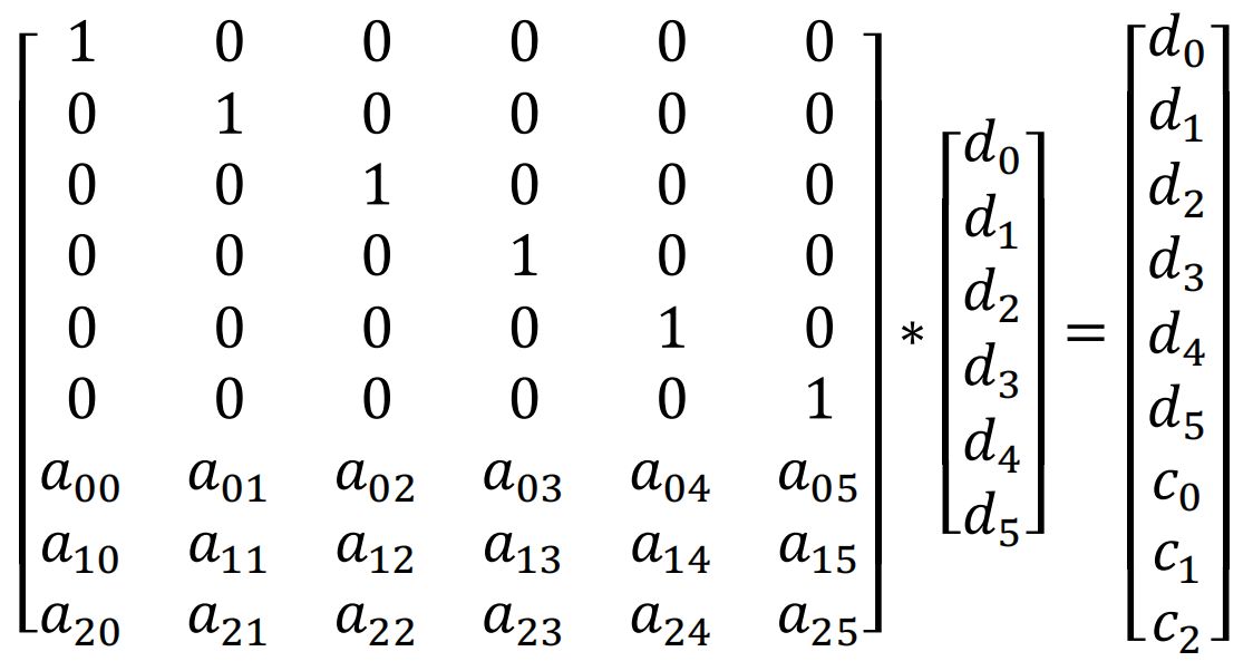
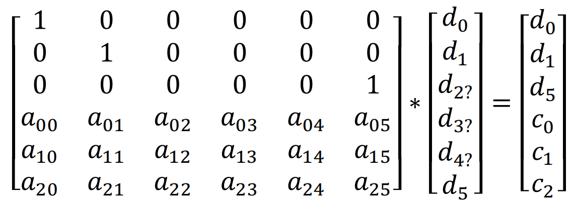
生成校验块即编码过程(encode)。对6个数据块依次取出byte, 即d₀,d₁,d₂,d₃,d₄,d₅。如下图所示，用编码矩阵(encodeMatrix)乘以对应的数据块,即得到原有的数据d₀,d₁,d₂,d₃,d₄,d₅和对应的校验字节c₀,c₁,c₂(编码过程)。对数据块的所有字节依次执行上述的操作就得到了校验块。

1.2 恢复数据块

恢复数据块的过程即解码过程(decode)。假如d2,d3,d4丢失了，我们需要通过d₀,d₁,d₅,c₀,c₁,c₂恢复d₂,d₃,d₄。在上面公式中删除对应的行，公式中用d_2?,d_3?,d_4?表示数据块丢失。有如下公式:

对上面的公式两侧都乘以裁剪后的矩阵的逆矩阵，这个逆矩阵即解码矩阵(decodeMatrix)。可以得到如下的公式:

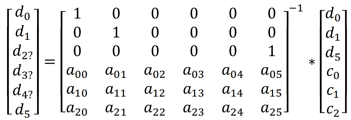
得到解码矩阵后其实计算过程与编码类似，只是输入为为d₀,d₁,d₅,c₀,c₁,c₂，输出为d₀,d₁,d₂,d₃,d₄,d₅。

2 关于矩阵

上一章节已经介绍了EC编解码的基本过程，但工程实现上让然会有一些问题需要解决。这一小节主要介绍一下关于矩阵方面的问题。

2.1 如何选择矩阵

根据第一小节的分析，编码矩阵是一个9 * 6的矩阵。而解码矩阵是在编码矩阵的基础上删除任意三行，然后再求逆的。因此我们定义编码矩阵的时候要保证，对于这个9 * 6的编码矩阵，任意删除三行得到的6 * 6的矩阵是一个可逆矩阵。
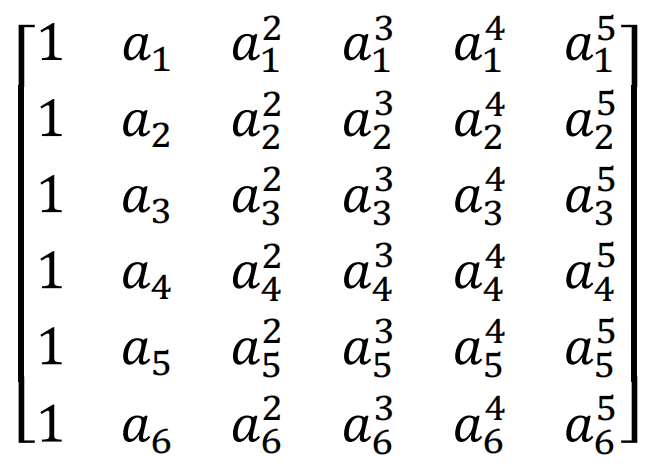
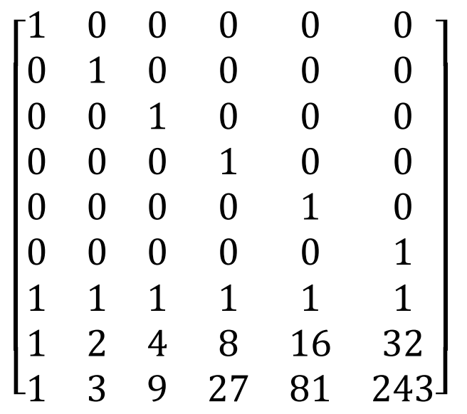
为了便于计算，编码矩阵的上半部分使用的是6 * 6 的单位矩阵，单位矩阵是可逆的，是满足条件的。接下来就是给下半部分的3 * 6的找到合理的矩阵。本文使用的是范德蒙矩阵。

由于MathType不支持新版Mac, 而且markdown经常因为调整不好乱码，这里的共识还是贴图吧…

如下为范德蒙矩阵的行列式:

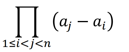
只要ai各不相等且不为0，则范德蒙矩阵一定可逆，意味着任意挑出3行向量，一定是线性无关的。那我们就挑出前三行，令a₁=1,a₂=2,a₃=3，便可以得到如下编码矩阵:

前面已经说明了前6行向量是互为线性无关，后3行向量也是互为线性无关的。如果在前6行中选取n行，在后三行中去6-n行，那么这6行向量还是线性无关的吗？假设n为5，由于后三行的没有元素为0，因此肯定是缺一个维度来保证线性相关。如果n为4和3也是同样的道理。因此这个9 * 6的矩阵随意挑出6行组成的6 * 6阶矩阵一定是可逆的。

2.2 高斯消元求逆

本文使用了容易理解的高斯消元法求逆(inverse)。假设当前6 * 6矩阵为A, 在右侧再拼接6 * 6的单位矩阵E，得到矩阵[A | E]。如果使用A^-1乘以这个矩阵，会得到[E|A^-1]。这样我们只需将A矩阵转化为单元矩阵，E矩阵自然就变成了A^-1。(高斯消元求逆)
对每一行行依次执行如下的过程:

(1) 对第i行, 找到第i行第i列的值。(Step1)
(2) 然后计算该值的乘法逆元。然后让该行的每个元素均乘以这个乘法逆元。(Step2)
(3) 对其他行j，使用第i行经过线性变换将地地j行第i列的值消为0。

经过这三步变换为，对于第i列，有且只有地i行的数据为1，其他均为0。对每一行均执行如下操作，左侧变得到了单位矩阵，右侧的结果也即A^-1。

对于有理数域中，乘以乘法逆元即除法，加上加法逆元即减法。这样描述对伽罗华域中的数学运算的描述更准确。

对于第0行计算的过程如下，其他行同理。

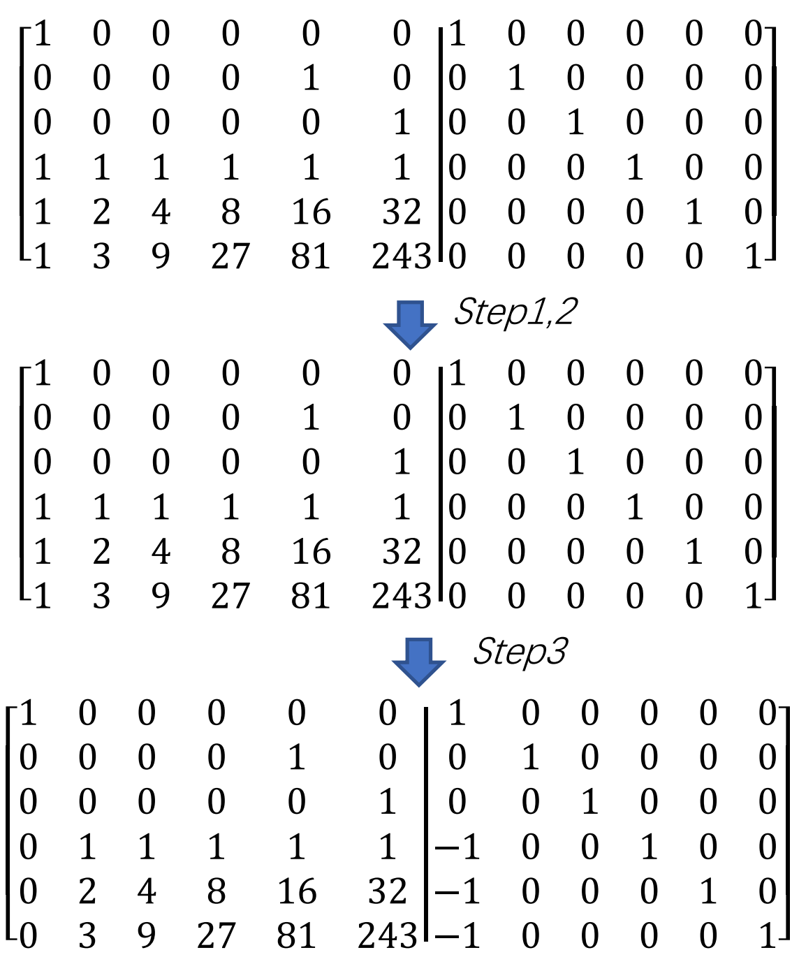
还有一种特殊的情况，譬如上述矩阵如果处理第2行。第2行和第2列的元素值为0，0是没有乘法逆元的。所以这时候就需要找到第2行下面的行中第2列不为0的情况，把该行加到第2行上，这样可以保证算法可运行(setup for step1)。其实移位可能更高效，但是为了便于理解，采用这样的方式。

3 伽罗华域

矩阵运算还存在一个问题，数据都是byte存储的，是一个0-255的数值。经过有理数运算后，数值是很容易越界的。因此我们需要一套新的计算体系同时满足以下两个条件:

该算法体系的值和计算得到的值只能是在有限的集合范围内，即不越界。
可以通过有限的运算恢复得到原有值，即可解码。

这就需要使用伽罗华有限域。伽罗华有限域可以保证任何计算得到的结果均在有限集合内，这满足了不越界的要求。另外伽罗华有限域的运算都有对应的逆运算。譬如对a，如果a乘以b，再乘以b的加法逆元，结果仍然是a。这满足了可解码的要求。

这里为了便于理解先简单的介绍GF(7)，然后再解释实际使用的GF(2⁸)。

本章并没有详细的证明。譬如将7扩张到无穷大的质数的时候，如何证明相应的定理为什么成立。事实上笔者也不知道，参考文献上也没有严谨的证明。也只是简单的说明了合数不能作为模数。但对于工程上有限的集合内，很容易通过穷举法来证明算法的可行性。

3.1 GF(7)

首先给出如下定义:

加法逆元: 给定x，如果存在x’，使得x+x’=x’+x=0，则称x’是x的加法逆元。
乘法逆元: 给定x，如果存在x’，使得x * x’=x’ * x=e，则称x’为x的乘法逆元。其中e为该群的单位元。对于GF(7)，e为1。

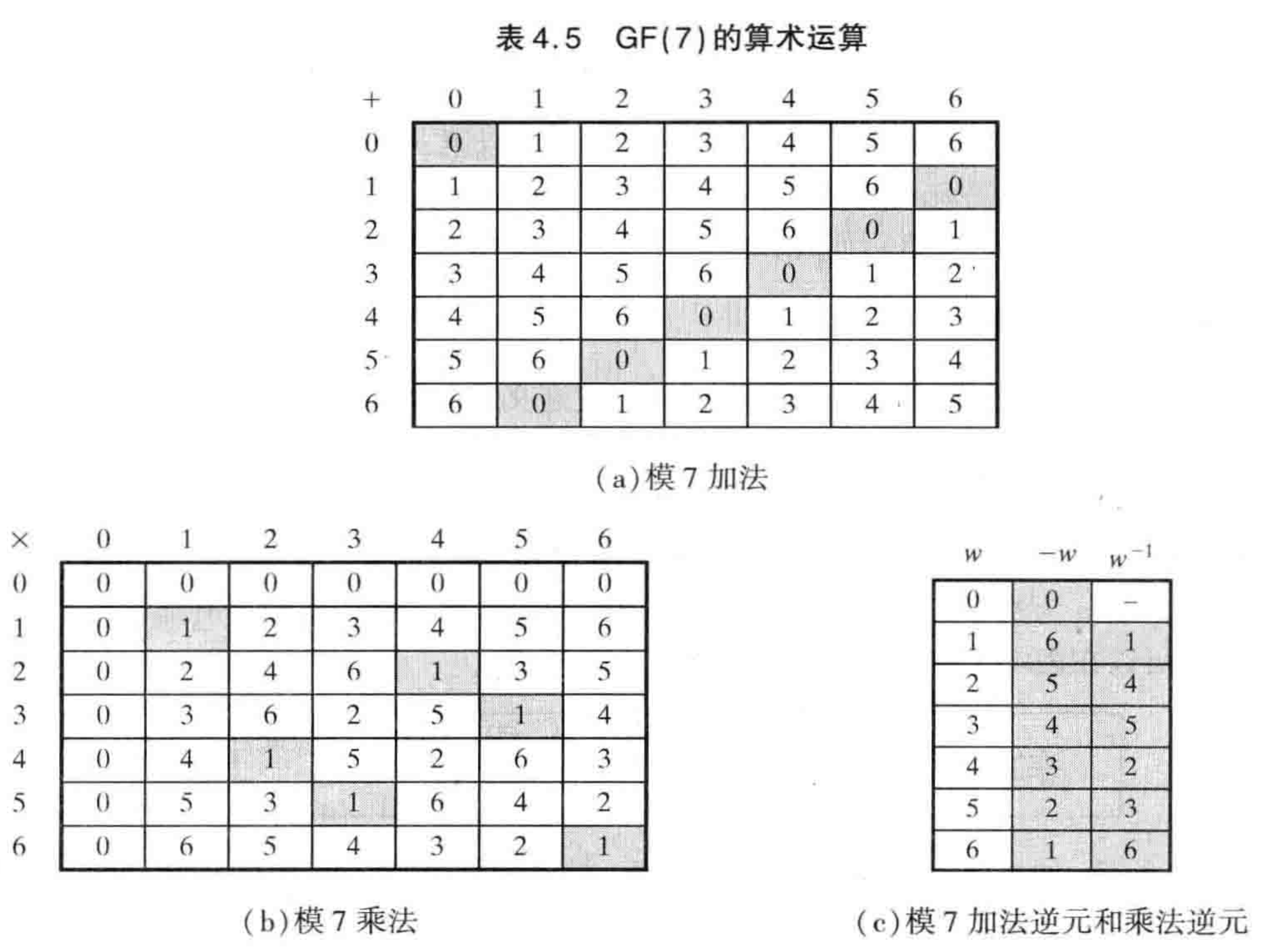
我们定义一种新的运算，即模7运算。对于加法和乘法运算，我们会将结果然后模7。譬如, 8 + 3 = 11 mod 7 = 4。8 * 3 = 24 mod 7 = 3。
对于加法逆元和乘法逆元，根据定义我们可以穷举加法和乘法计算，根据结果得到对应的逆元。譬如, 4 + 3 = 7 mod 7 = 0，我们就说4和3互为加法逆元。2 * 4 = 8 mod 7 = 1，我们就说2和4互为乘法逆元。
下表穷举了GF7的所有加法和乘法运算，根据码表也得到了GF(7)下所有元素对应的加法逆元和乘法逆元。

来看下是否满足我们的要求，不越界在定义上就满足了。可解码的特点，我们随机指定数组假设为5，用5乘以3在乘以3的乘法逆元5, 得到的值为5 * 3 * 5 = 75 mod 1 = 5。事实上根据乘法交换律很容易证明这个。对于加法逆元的解码同理。

3.2 GF(2⁸)

3.2.1 基本原理

实际的数字存储的值是0-255, 那么是否意味着我们可以直接使用GF(256)呢? 答案是不可以的。因为256是合数，譬如16 * 16 = 256 mod 256 = 0，那么16就不存在乘法逆元，也就难以进行边界吗。
因此需要引入多项式的运算，且要求同指数幂下遵循GF(2)。模数为不可约多项式。对于不可约多项式a, 无法找到两个不为1的多项式b和c使得b * c = a。可以使用穷举法得到每个多项式的加法逆元和乘法逆元。事实上只要集合内的每个元素都有1对1对应的乘法逆元，就可以满足我们的要求。文献1的表4.6也通过穷举证明了GF(2³)的有效性。
多项式的计算与对byte的编码有什么关系呢？由于多项式的同指数幂是GF(2)，也就意味着对于多项式a₀ + a₁x + a₂x² + a₃x³ + a₄x⁴ + a₅x⁵ + a₆x⁶ + a₇x⁷ ，a_i 为0和1。如果a₀为第0位，a₁为第1位，依次类推，这组系数就是一个byte。这样就把要存储的byte与多项式运算结合了。

3.2.2 计算

本章主要介绍如何计算GF(2⁸)。对于加法和乘法，我们直接使用多项式运算。对于加法逆元和乘法逆元，我们穷举加法和乘法运算，然后通过码表来得到加法和乘法逆元。
本文的算法的不可约多项式为x⁸ + x⁴+ x³ + 1。
f(x) = x⁶ + x⁴+ x² + x + 1, g(x) = x⁷ + x + 1
对于加法, 指数幂执行GF(2)运算，G(2)运算实际上就是异或。得到f(x)+g(x)= x⁷ + x⁶ +x⁴+ x² + 1。实际可以理解为f(x)对应的二进制0b01010111与g(x)对应的二进制0b10000011进行按位的异或计算。(GF(2⁸))
对于乘法, 先考虑h(x) = a₀ + a₁x + a₂x² + a₃x³ + a₄x⁴ + a₅x⁵ + a₆x⁶ + a₇x⁷, 计算 h(x) * x = (a₀x + a₁x² + a₂x³ + a₃x⁴ + a₄x⁵ + a₅x⁶ + a₆x⁷ + a₇x⁸ ) mod (x⁸ + x⁴+ x³ + x + 1)。存在两种情况

(1) a₇ 等于 0
那么该式已经不可约，因此h(x) * x= a₀x + a₁x² + a₂x³ + a₃x⁴ + a₄x⁵ + a₅x⁶ + a₆x⁷。也就意味着[a₇a₆a₅a₄a₃a₂a₁a₀] * [00000010] = [a₆a₅a₄a₃a₂a₁a₀0]，即向左移动一位。(a₇ 等于 0)
(1) a₇ 不等于0
h(x) * x = (a₀x + a₁x² + a₂x³ + a₃x⁴ + a₄x⁵ + a₅x⁶ + a₆x⁷ + x⁸) mod (x⁸ + x⁴+ x³ +x+ 1) = a₀x + a₁x² + a₂x³ + a₃x⁴ + a₄x⁵ + a₅x⁶ + a₆x⁷ + x⁸ - x⁸ - x⁴ - x³ -1 = 1 + (a₀+1)x + a₁x² + (a₂+1)x³ + (a₃+1)x⁴ + a₄x⁵ + a₅x⁶ + a₆x⁷。以为意味着[a₇a₆a₅a₄a₃a₂a₁a₀] * [00000010] = [a₆a₅a₄a₃a₂a₁a₀0] ^ [00011011]。即左移一位后，在于不包含最高位系统的字节进行异或。(a₇ 不等于 0)

这里减法为加法逆元，对于GF(2)，加法逆元就是自己。

f(x) * g(x) = ((x⁶ + x⁴+ x² + x + 1) * ( x⁷ + x + 1))。我们可以把他分解为一下三个运算之和。

(1) (x⁶ + x⁴+ x² + x + 1) * x⁷
(2) (x⁶ + x⁴+ x² + x + 1) * x
(3) (x⁶ + x⁴+ x² + x + 1) * 1
对于(2)在前面已经介绍了，对于(3)实质上不用计算。对于(1), 我们可以使用(2)的计算方法进行递归计算(fxxn)。然后分别计算的三个值进行相加便得到了最终的结果(_mul)。

至此，ErasureCode算法的所有问题都已经得到了解释。本文以自顶向下的方式描述了如何从理论到实践来实现ErasureCode算法。完整的代码见SimpleErasureCode。

参考文献:

[1]William Stallings. 密码编码学与网络安全原理与实践第六版[M] 第四章
[2]https://drmingdrmer.github.io/tech/distributed/2017/02/01/ec.html

2025-02-07

title: 机器学习-2.8-监督学习之k近邻算法
date: 2017-10-15 20:29:06
tags: [机器学习]

K近邻算法

K近邻算法是一种常用的监督学习算法。其工作机制非常简单: 给定测试样本，基于某种距离度量找到与测试样本最近的k个训练样本，然后可以根据k个样本决定分类。譬如可以选择k个样本中最多的测试样本进行分类。

下面我们使用k近邻算法识别手写数字。手写数字为一个32*32维的向量，我们可以把它看成一个1024维的向量。然后任意两个样本的距离完全可以通过计算1024维上的两个点之间的距离获得，然后我们可以找到与测试样本距离最近的的10个样本，其中最多的分类我们认为他就是测试样本的分类。具体代码如下：

import numpy as np
import os
from numpy import linalg

global g_train
global g_label

def makeTrain(dir):
  dirs=os.listdir(dir)
  files = filter(lambda item:not os.path.isdir(item), dirs)
  mat = []
  label = []

  for file in files:
    arr = []
    f = open(dir+"/"+file)
    while True:
      line = f.readline()
      if not line:
        break
      for i in range(len(line)-1):        # line[len(line)]='\n'
        arr.append(int(line[i]))
    mat.append(arr)
    label.append(int(file.split("_")[0]))
  return (np.array(mat),np.array(label))

def testClassify(dir):
  dirs=os.listdir(dir)
  files = filter(lambda item:not os.path.isdir(item), dirs)
  mat = []
  right=0
  wrong=0
  for file in files:
    arr = []
    f = open(dir+"/"+file)
    while True:
      line = f.readline()
      if not line:
        break
      for i in range(len(line)-1):        # line[len(line)]='\n'
        arr.append(int(line[i]))
    mat.append(arr)
    testLabel = file.split("_")[0]
    label=classify(np.array(arr),10)
    if testLabel == label:
      right=right+1
    else:
      wrong=wrong+1
  print("right=",right,", wrong=",wrong)

def classify(vec,k):
  # 计算各个训练数据与测试数据的距离
  m = len(g_label)
  dis = []
  for i in range(m):
    dis.append([linalg.norm(vec-g_train[i]),g_label[i]])
  dis = sorted(dis, key=lambda v:v[0])

  # 计算相似度最高的k个值，这里写入map做累积
  dic = {}
  for j in range(k):
    if not str(dis[j][1]) in dic:
      dic[str(dis[j][1])]=1
    else:
      dic[str(dis[j][1])]=dic[str(dis[j][1])]+1
  return max(dic.items(), key=lambda x: x[1])[0]

if __name__ == "__main__":
  # 1 formate trainning date
  (g_train,g_label) =makeTrain("/Users/zcy/Desktop/study/git/mlearning/res/trainingDigits1")

  # 2 test
  testClassify("/Users/zcy/Desktop/study/git/mlearning/res/testDigits1")

计算946个测试样本集，有926个为正确计算，20个为错误计算，识别为97.89%

2023-12-25

RSS-Remote Merge Design

1 Default shuffle

Note: The first chapter briefly introduces the principle of default shuffle, with the purpose of find where local disks are used, then design remote merge. If you know enough, you can ignore this part.

We will analyze the shuffle of MapReduce, Tez, and Spark in turn.

1.1 MapReduce

Map writes the record to the memory. When the memory exceeds the threshold, the memory data is spilled to the disk file, and the Record is written to the disk file in order of partitionid+key. After Map has processed all records, it will spill the data currently in memory to a disk file. Then read all the files spilled to the disk and merge them in the order of partitionid+key to get the sorted Records.

Note: The purpose of sorting according to partitionid is that when the Reduce side obtains the data from the Map side, it should be read as sequentially as possible. For MR, Tez, and Spark, regardless of whether they are sorted or not, as long as there are partitioned, they need to be sorted according to partitionid.

The reduce will pull the records of the corresponding partition remotely or locally from the Map, which is called MapOutput. Under normal circumstances, the memory will be used directly. If the memory exceeds the threshold, these records will be written to the disk. Then the reduce will perform merge operations on MapOutputs using minimum heap K-way merge sorting to obtain globally sorted records. During the Merge process, temporary results may be spilled to disk because the memory exceeds the threshold. In addition, if there are too many files spilled to disk, additional merges will be triggered.

1.2 Tez

There are two cases of tez: (1) ordered io (2) unordered io.

Ordered io is the same as MapReduce and so ignore it here.

Unordered io is generally used in hashjoin and other situations where keys are not required for sorting. Non-sorted io adopts a ready-to-use solution. Map writes the Record directly to the file or writes it to the file through cache. The Reduce side can also read and use it when reading data.

1.3 Spark

Spark’s shuffle is more complex and more reasonable. Some tasks do not require sort and combine, so spark users can determine the shuffle logic according to their needs.

1.3.1 Shuffle write operation

When writing shuffle data, three writers are supported:

(1) BypassMergeSortShuffleWriter

A temporary file is generated for each partition. When writing record, find the corresponding partition and write it directly to the corresponding temporary file. Then when all data is processed, these temporary files are written to a final file in order of the partitions, and the temporary files are deleted.

(2) UnsafeShuffleWriter

UnsafeShuffleWriter mainly implements specific logic through ShuffleExternalSorter. When writing a Record, the serialization operation is performed directly and the serialized bytes are copied to the requested memory. At the same time, the address and partition of the record will also be recorded into the memory (inMemSorter).

When the memory reaches the threshold, spill operation will be performed. Based on the information in memory (inMemSorter), we can easily get a Record sorted by partition and write it to a file.

When all Records are processed, we will spill the records currently in memory into the file. Finally, all spilled files are aggregated once. Since the previously spilled files have been sorted according to the partition, we can copy the corresponding copies of all the spilled files to the final file in the order of the partitions. The final file obtained in this way is the partition-sorted file.

(3) SortShuffleWriter

SortShuffleWriter mainly implements specific logic through ExternalSorter. ExternalSorter decides whether to combine and sort based on the user’s needs.

When writing record, it will be inserted directly into memory. If combine is required, the memory architecture is map, otherwise it is buffer.

If the current evaluation memory is greater than the threshold, the spill operation will be triggered. During the spill operation, the Record will be spilled to the disk. This process requires sorting. The specific comparator will use different values according to different user needs. If keyordering is set, it will be sorted by key. If keyordering is not set, but aggregator (i.e. combine) is set, the keys are sorted according to the hashcode of key, thus ensuring that the same keys are organized together to facilitate combine operations. If neither keyordering nor aggregator is set, it will be sorted according to partition.

When all Records are written, the spill files need to be read and merged into a globally ordered file.

Comparison of three writers

writer	advantages	disadvantages	scene
BypassMergeSortShuffleWriter	(1) Only serialized once. (2) Using hashmap-like data structure, inserting data is fast.	(1) Combine and sort are not supported (2) Each partition must generate a temporary file, which will generate too many temporary files.	Suitable for situations where the number of partitions is small (default is less than or equal to 200) and there is no combine.
UnsafeShuffleWriter	(1) Only serialized once. (2) The number of files spilled to disk is limited and is no longer based on the number of partitions, and can support larger partitions.	(1) Combine, sort is not supported (2) The writing order Record order will be disrupted, and supportsRelocationOfSerializedObjects is required.	Applicable to situations where combine does not exist, and supportsRelocationOfSerializedObjects is true, and the maximum number of supported partitions is 16777216.
SortShuffleWriter	(1) Supports combine, sort (2) Suitable for all scenarios (3) The number of files spilled to disk is limited	(1) Multiple serializations are required	Suitable for all scenarios.

1.3.2 shuffle read

Currently there is only one implementation of BlockStoreShuffleReader. The implementation is similar to MapReduce.
The reduce will pull the records of the corresponding partition remotely or locally from the map. Under normal circumstances, it will be written directly to the memory, but if the block size to be obtained exceeds the threshold, will use disk.
Then it will be decided according to the user’s needs whether to combine or sort, and finally form a record iterator required by the user.
Combine and sort use ExternalAppendOnlyMap and ExternalSorter respectively. When the memory exceeds the threshold, the data will be spilled to the local disk.

1.4 Summary

(1) About the semantics of each framework

For MapReduce and the ordered io of Tez, it is a special case of spark sorting. For Tez’s unordered io, it is essentially a special case of spark’s non-sorting. In essence, the semantics of each framework are the same, and spark is more general.

(2) Where will generate local disk files?

After analyzing the three computing frameworks, we learned that the following processes will use disks:

(1) Map may generate intermediate temporary files because the memory exceeds the threshold.
(2) The map will eventually generate disk files to provide shuffle services.
(3) When reduce pulls records, disk files may be generated because the threshold is exceeded.
(4) When merging on the reduce side, temporary disk files may be generated for global sorting.

In fact, uniffle has solved (1), (2). For (3), if the parameters are adjusted effectively, it is difficult to generate disk files. In fact, only (4) needs to be discussed in this article.

2 Plans

In order to solve the problem that Merge on the Reduce side may spill to disk, there are two main solutions:

(1) Merge on Shuffle Server
(2) Reduce side Merge on demand

2.1 Option 1: Merge on ShuffleServer

Move the merge process of reduce to the ShuffleServer side. ShuffleServer will merge the locally sorted Records sent from the map side into a globally sorted records sequence. The reduce side reads directly in the order of the records sequence.

Advantages: Does not require too much memory and network RPC.
Disadvantages: Shuffle Server needs to parse Key, Value and Comparator. The Shuffle side cannot combine.

2.2 Option 2: On-demand Merge on the Reduce side

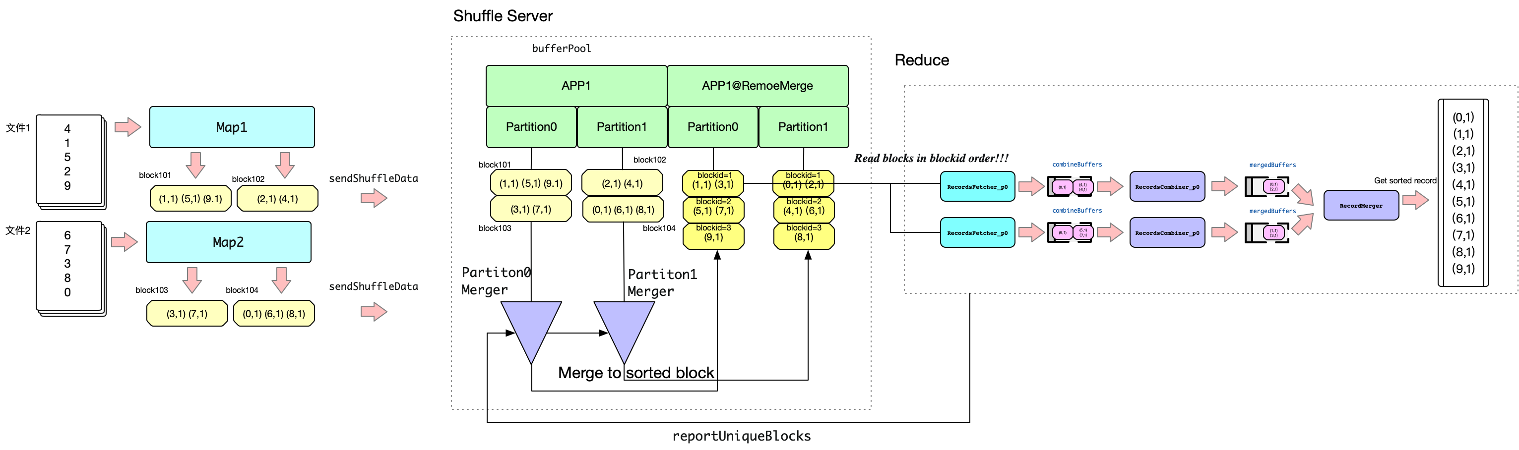
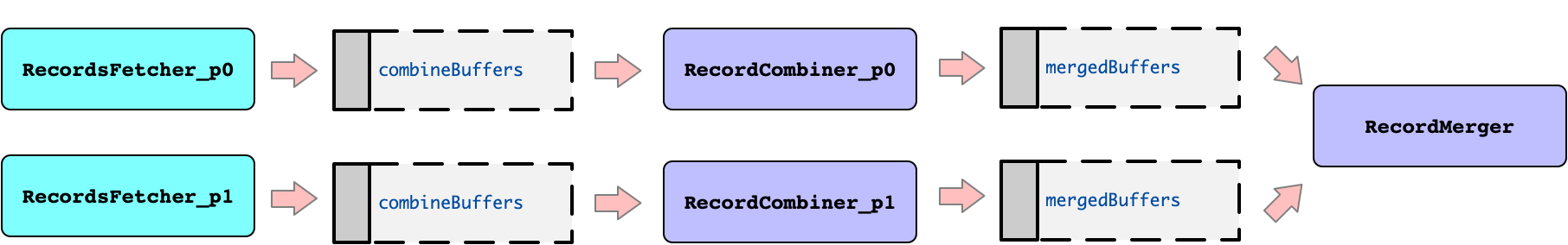
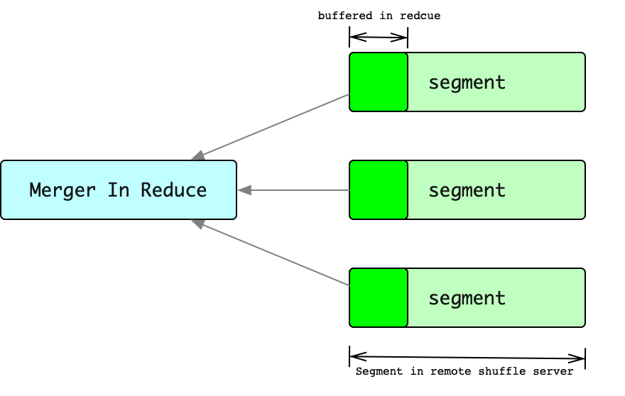
Since the memory on the reduce side is limited, in order to avoid spilling data to disk when merging on the reduce side. When reduce obtains segment, it can only read part of the buffer of each segment, and then merge all the buffers. Then when the partial buffer reading of a certain segment is completed, the next buffer of this segment will continue to be read, and this buffer will continue to be added to the merge process. There is a problem with this. The number of times the Reduce side reads data from ShuffleServer is approximately segments_num * (segment_size / buffer_size), which is a large value for large tasks. Too many RPCs means decreased performance.

The segment here refers to the sorted record collection, which can be understood as the block in which the records have been sorted according to key.

Advantages: Shuffle Server does not need to do anything extra.
Disadvantages: Too many RPCs.

**This article chooses option 1, and the following content mainly discusses option 1. **

3 Demand analysis

3.1 What types of tasks require remote merge?

Currently, uniffle’s map-side no longer spill disk. This article mainly considers the situation on the reduce. Mainly divided into the following situations:

(1) For spark’s non-sorted, non-aggregated, tez unordered io. It does not require any global aggregation and sorting operations, and only requires very little memory. The current version of uniffle will not use disk if related settings are reasonable. Just use the current uniffle solution. This article will not discuss this aspect.
(2) For spark sorting or aggregation tasks, tez ordered io, mapreduce, due to the need for global sorting or aggregation, the memory may not be enough, and the record may be spilled to the disk. This article mainly discusses this situation.
**In summary, it can be seen that remote merge is only used for shuffles that require sorting or aggregation. **

3.2 How does ShuffleServer sort?

For sorting, map is generally sorted to obtain a set of partially sorted records, which is called segment here. Then reduce will obtain all segments and merge them. Spark, MR, and Tez all use minimum heap K-way merge sorting. This method can still be used for remote sorting.

BufferManager and FlushManager maintain block information in memory and disk. We only need to add MergeManager to ShuffleServer and merge the blocks under the same Shuffle to obtain globally sorted Records.

Introducing sorting on the ShuffleServer produces a side effect: the Shuffle’s KeyClass, ValueClass and KeyComparator need to be passed to ShuffleServer.

3.3 How does ShuffleServer combine?

Combine is generally a user-defined operation, so ShuffleServer is prohibited from performing combine operations. If combine is performed on the Reduce side, wouldn’t it violate our theme of avoiding spill to disk on the task side? In fact we don’t have to use ExternalAppendOnlyMap for combine. If the Records obtained from ShuffleServer are sorted by key, it means that the same keys have been organized together, and only a small amount of memory is needed to combine.

3.4 How does Writer write?

Just write it the way we have it.

3.5 How does Reader read?

Currently, Uniffle’s shuffle reader uses blockid as the read mark, which makes it easy to verify whether an accurate and complete records are obtained. For remote merge, MergeManager has merged the original Block collection into a new sequence sorted records by key. Therefore, the blockid generated by the map segment cannot be used:
We will use a new way to read Records. When MergerManager performs global Merge, an index will be generated. Reader will read according to this index.

Note: In principle, using key as a read index is more semantic, and the first version of the demo program was also implemented by this way. However, this proposal was not friendly enough to deal with the problem of data skew, so gave up the plan.

4 Scheme Design

4.1 Basic procedures for RemoteMerge

The following introduces the process of Remote Merge:

(1) Register
When AM/Driver calls the registerShuffle method, it will additionally register keyClass, valueClass and keyComparator. This information is mainly used by ShuffleServer to parse and sort the Record during merging.
(2) sendShuffleData
The sendShuffleData logic is basically consistent with existing RSS tasks. The only difference is the use of unified serializers and deserializers, which ensures that ShuffleServer can parse the Record normally no matter which framework it is.
(3) buffer and flush
The shuffle server will store the data in the cache, or cache it to the local file system or remote file system through the flush manager. The logic of the original ShuffleServer is still reused here.
(4) reportUniqueBlocks
A new API is provided, reportUniqueBlocks. The Reduce end will deduplicate the blocks generated by the map, and then send the valid block set to ShuffleServer through reportUniqueBlocks. After ShuffleServer receives a valid blocks collection, it will trigger Remote Merge. The results of Remote Merge will be written to the bufferPool like a normal block, and may be flushed to disk when necessary. The result generated by RemoteMerge is an ordinary block, but for convenience of explanation, it is called merged block here. The merged block records the results sorted by key, so when reading the merged block, you need to read it in ascending order in the order of blockid.
(5) getSortedShuffleData
Reduce will read merged blocks in the order of block serial numbers, and then choose when to use them for reduce calculations based on certain conditions.

4.2 Analyze the process from the perspective of Record

We can use WordCount as an example to explain the flow of record in the entire process. In this example, there are two partitions and one reduce, that is, one reduce processes the data of two partitions.

(1) MAP side
After the document data is processed on the map side, it will be sorted. For Map1, since there are two partitions, records with odd numbers as keys will be written to block101, and records with even numbers as keys will be written to block102. The same goes for Map2. Note that the Records in the block here are all sorted.
(2) Map side sends data
The map side sends the block to ShuffleServer through sendShuffleData, and ShuffleServer stores it in the bufferPool.
What I mean here is that when registering, the app named APP1 will also be registered, and the app named APP1@RemoteMerge will also be registered, which will be introduced later.
(3) ShuffleServer side Merge
After reduce is started, reportUniqueBlocks will be called to report the available block set, and the corresponding partition in ShuffleServer will be triggered to merge. The result of Merge is a globally sorted record collection under this partition.
Then the question is where are the results of merge stored? The merge process occurs in memory. Whenever a certain number of records are merged, the results are written to a new block. In order to distinguish it from the original appid, this group of blocks will be managed in an appid ending with “@RemoteMerge”. The blockid of this new group of blocks increases from 1 and is sorted globally. That is, the records inside each block are sorted, and the records with blockid=1 must be less than or equal to the records with blockid=2.
(4) Reduce end reading
According to the previous analysis, the reduce side only needs to read the block managed by the appid ending with “@RemoteMerge”. When reduce reads a block, it starts from the block with blockid=1 and reads in the order of blockid. We know that when reduce performs calculations, it is calculated in order. Since the data we obtain on the ShuffleServer side is already sorted, we only need to obtain a small amount of data from the ShuffleServer side each time. This enables on-demand reading from the ShuffleServer side, which greatly reduces memory usage.
There are two special situations here, detailed in 5.5.

5 Plan

5.1 Unified serializer

Since Merge needs to be performed on the ShuffleServer side, a unified serializer that is independent of the computing framework needs to be extracted. Two types of serializers are extracted here: (1) Writable (2) Kryo. Writable serialization is used for classes that handle the org.apache.hadoop.io.Writable interface, used in the MR and TEZ frameworks. Kryo can serialize most classes and is generally used in the Spark framework.

5.2 RecordsFileWriter/RecordFileReader

Provides abstract methods for processing Records

5.3 Merger

Provides basic Merger service to merge multiple data streams according to key. Minimum heap K-way merge sorting is used to merge and sort the data streams that have been partially sorted.

5.4 MergeManager

Used to merge Records on the server side.

5.5 Tools for reading sorted data

Generally speaking, when the Reduce side reads data, it can be sent directly to downstream calculations. But there are two special situations:
(1) For situations where it is necessary to combine in Merge, we need to wait for all the same keys to arrive before combining, and then send them to the downstream.
(2) For spark and tez, the reduce end can read data from multiple partitions. Therefore, we need to merge the data of multiple partitions again on the reduce side, and then send it to the downstream.
RMRecordsReader is a tool for reading sorted data. The general structure is as follows:

The figure depicts a situation where a single Reduce processes two partitions. The RecordsFetcher thread will read the block of the corresponding partition and then parse it into Records. Then send it to combineBuffers. RecordCombiner reads Records from combineBuffer. When all records of a certain key are collected, a combine operation is performed. The result will be sent to mergedBuffer. RecordMerge will obtain all mergedBuffers and then merge and sort them again in memory. Finally, the global sorting results are obtained for downstream.

5.6 Framework adaptation

Compatible with MR, Tez, and Spark architectures.

I has used online application to conduct large-scale stress testing on MR and Tez. Spark has currently only tested some basic examples and still needs a lot of testing.

5.7 Isolated classloader

For different versions of keyclass, valueclass and comparatorclass, use isolated classloaders to load them.

Chinese version document: https://zhengchenyu.github.io/2023/12/25/RSS-%E8%BF%9C%E7%A8%8BMerge%E7%9A%84%E8%AE%BE%E8%AE%A1/

2023-12-25

RSS-远程Merge的设计

1 默认的shuffle

注: 第一节简单介绍了主流框架默认的shuffle的原理，目的为了那里会使用本地磁盘，从而设计远程Merge。如果足够了解，可以忽略这部分内容。

我们依次对MapReduce, Tez, Spark的shuffle进行分析。

1.1 MapReduce

Map将Record写入到内存，当内存超过阈值的时候，会将内存的数据spill到磁盘文件中，按照partitionid+key的顺序依次将Record写入到磁盘文件。当Map处理完所有Record后, 会将当前内存中的数据spill到磁盘文件。然后读取所有的spill到磁盘的文件，并按照partitionid+key的顺序进行merge，得到排序的Records。

注: 按照partitionid排序的目的是Reduce端从Map端获取的数据的时候，尽可能顺序读。对于MR、Tez、Spark, 无论是否排序，只要有分区，都需要按照partitionid进行排序。

Reduce端会从Map端以远程或本地的方式拉取对应分区的Records，称之为MapOutput。正常情况下会直接使用内存，如果内存超过阈值会将这些Records写入到磁盘。然后Reduce端会对所有MapOutput使用最小堆K路归并排序进行一些Merge操作，得到全局排序的Reccords。Merge的过程中，可能会因为内存超过阈值，会将临时的结果spill到磁盘。另外如果spill到磁盘的文件过多，也会触发额外的merge。

1.2 Tez

Tez的情况略微复杂。Tez分为ordered io和unordered io。

ordered io与MapReduce相同，不再展开分析。

unordered io一般用于hashjoin等不需要key进行排序的情况。非排序的io采用来之即用方案。Map直接将Record写入文件或者通过缓存在写入文件。Reduce端也是读数据的时候也是读之即用。

1.3 Spark

spark的shuffle更复杂，也更合理。部分任务是不需要sort和combine的，因此spark用户可以需求决定shuffle的逻辑。

1.3.1 Shuffle写操作

写shuffle数据的时候，支持三种writer:

(1) BypassMergeSortShuffleWriter

为每个partition都生成一个临时文件。在写Record的时候，找到对应的分区直接写入对应的临时文件。然后当所有数据都处理完成后，将这些临时的文件按照分区的顺序依次写入到一个最终的文件，并删除临时文件。

(2) UnsafeShuffleWriter

UnsafeShuffleWriter主要通过ShuffleExternalSorter来实现具体的逻辑。当写Record的时候，直接序列化操作，并将序列化的字节拷贝到申请的内存中。同时也会将Record的地址和分区记录到内存中(inMemSorter)。

当内存的Record达到阈值的时候，会进行spill操作。根据内存(inMemSorter)中的信息，我们很容易得到一个按照分区排序的Record，并写到文件中。

当处理完所有Record，我们会把当前内存中的Records spill到文件中。最后对所有spilled文件进行一次聚合。由于之前spilled的文件已经是按照分区排序的，所以我们可以按照分区的顺序依次将所有spill的文件的对应自己拷贝到最终文件。这样得到的最终文件即为分区排序的文件。

(3) SortShuffleWriter

SortShuffleWriter主要通过ExternalSorter来实现具体逻辑。ExternalSorter根据用户的需求决定是否combine和sort。

当写Record的时候，会直接插入到内存中。如果需要combine，内存架构是map，否则是buffer。

如果当前评估内存大于阈值会触发spill操作。spill操作的时候，会将Record，然后spill到磁盘。这个过程是需要进行排序的。而具体的比较器会根据用户需求的不同使用不同的值。如果设置了keyordering会按照key进行排序。如果没有设置keyordering，但是设置了aggregator(即combine)，则按照key的hashcode进行排序，这样保证相同的key组织一起，便于combine操作。如果keyordering和aggregator都没有设置，则会按照partiton进行排序。

所有Record都写完时，需要读取spill的文件，并合并成一个全局有序的文件。

三种writer的比较

writer	优点	缺点	场景
BypassMergeSortShuffleWriter	(1) 只经过一次序列化。 (2) 采用类hashmap的数据结构，插入数据快。	(1) 不支持combine (2) 每个分区都要对应生成一个临时文件，会产生过多的临时文件。	适合分区数较少(默认小于等于200)且没有combine的的情况.
UnsafeShuffleWriter	(1) 只经过一次序列化。 (2) spill到磁盘的文件数目有限，不再基于分区数，可以支持更大的分区。	(1) 不支持combine (2) 写入顺序Record顺序会打乱，要求supportsRelocationOfSerializedObjects。	适用于没有combine的情况，且支持supportsRelocationOfSerializedObjects，并且支持最大支持分区数为16777216。
SortShuffleWriter	(1) 支持combine (2) 适合于所有场景 (3) spill到磁盘的文件数目有限	(1) 需要进行多次序列化	适用于所有场景。

1.3.2 shuffle读

当前只有BlockStoreShuffleReader一个实现。实现与MapReduce类似。
Reduce端会从Map端以远程或本地的方式拉取对应分区的Records。正常情况下会直接写到内存中，但如果要获取的block大小超过阈值则会使用磁盘。
然后会根据用户的需求决定是否进行combine或sort，最终形成一个用户要求的record iterator。
combine和sort分别使用了ExternalAppendOnlyMap和ExternalSorter，当内存超过阈值后，会将数据spill到本地磁盘中。

1.4 总结

(1) 关于各个框架语义

对于MapReduce和Tez的ordered io, 实质就是spark的排序的特例。对于Tez的unordered io，实质上就是spark的非排序的特例。实质各个框架上语义是相同的, spark更加泛化。

(2) 哪里会产生本地磁盘文件?

分析三种计算框架后，我们得知如下过程会使用磁盘:

(1) Map由于内存超越阈值，可能会产生中间的临时文件。
(2) Map端最终必然会产生磁盘文件，用于提供shuffle服务。
(3) Reduce拉取records时候，可能因为超越阈值，产生磁盘文件。
(4) Reduce端Merge的时候，可能会产生临时的磁盘文件，用于全局排序。

而事实上, uniffle已经解决(1), (2)。对于(3), 如果有效的调整参数，是很难产生磁盘文件的。事实上只有(4)是本文需要讨论的。

2 方案的选择

为了解决在Reduce端Merge可能会spill到磁盘的问题，主要有两个方案:

(1) Shuffle Server端进行Merge
(2) Reduce端按需Merge

2.1 方案1: ShuffleServer端进行Merge

将Reduce的Merge过程移到ShuffleServer端，ShuffleServer会对Map端发来的局部排序后的Records进行Merge，合并成一个全局排序的Records序列。Reduce端直接按照哦Records序列的顺序读取。

优点: 不需要过多内存和网络RPC。
缺点: Shuffle Server端需要解析Key, Value和Comparator。Shuffle端不能combine。

2.2 方案2: Reduce端按需Merge

由于Reduce端内存有限，为了避免在Reduce端进行Merge的时候spill数据到磁盘。Reduce在获取Segment只能读取每个segment的部分buffer，然后对所有buffer进行Merge。然后对然后当某一个segment的部分buffer读取完成，会继续读取这个segment的下一块buffer，将这块buffer继续加到merge过程中。这样有一个问题，Reduce端从ShuffleServer读取数据的次数大约为为segments_num * (segment_size / buffer_size)，对于大任务这是一个很大的值。过多的RPC意味着性能的下降。

这里的segment是指排序后record集合，可以理解为record已经按照key排序后的block。

优点: Shuffle Server不需要做额外的任何事情。
缺点: 过多的RPC。

本文选择方案1，接下来的内容主要针对于方案1进行讨论。

3 需求分析

3.1 哪类任务需要远程merge?

当前uniffle的map端操作已经不再需要磁盘操作。本文主要考虑reduce端的情况。主要分如下几种情况:

(1) 对于spark的非排序且非聚集、tez unordered io，Record是来之即用的，不需要有任何的全局的聚合和排序操作，只需要非常少的内存。当前版本的uniffle在内存设置合理的情况下是不会使用磁盘的。使用当前uniffle的方案即可。本文不会讨论这方面的内容。
(2) 对于spark的排序或聚集任务、tez ordered io、mapreduce，由于需要全局排序或聚集，内存可能不够用，可能会将Record spill到磁盘。本文主要讨论这种情况。
综上可知，remote merge仅用于需要排序或聚集的shuffle。

3.2 ShuffleServer如何进行排序?

对于排序类的操作，一般会在Map进行排序得到一组局部排序的记录，这里称之为segment。然后Reduce会获取所有的segment, 并进行归并，Spark, MR, Tez都是用了最小堆K路归并排序。远程排序依旧可以使用这种方式。

BufferManager和FlushManager维护着block在内存和磁盘中的信息。我们只需要在需要在ShuffleServer中新增MergeManager，并将同一个Shuffle下的block进行Merge，得到全局排序的Records即可。

在ShuffleServer端引入排序后产生一个副作用: 即需要将该Shuffle的KeyClass和ValueClass以及KeyComparator传递给ShuffleServer。

3.3 ShuffleServer禁止combine

Combine一般都是用户自定义的操作，因此禁止ShuffleServer端进行Combine操作。

4 架构设计

4.1 RemoteMerge的基本流程

下面介绍一下Remote Merge的流程:

(1) 注册
AM/Driver调用registerShuffle方法，会额外注册keyClass, valueClass和keyComparator. 这些信息主要用于ShuffleServer在合并的时候对Record进行解析和排序。
(2) sendShuffleData
sendShuffleData逻辑与现有的RSS任务基本保持一致。唯一区别是使用统一的序列化器和反序列化器，这样可以保证无论是哪一种框架，ShuffleServer都可以正常的解析Record.
(3) buffer and flush
shuffle server端会将数据存在缓存中，或者通过flush manager缓存到本地文件系统或远程文件系统。这里还是复用原来的ShuffleServer的逻辑。
(4) reportUniqueBlocks
提供了一个新的API, 即reportUniqueBlocks。Reduce端会根据map产生的block进行去重，然后将得到有效block集合通过reportUniqueBlocks发送给ShuffleServer。ShuffleServer收到有效的blocks集合后，会触发Remote Merge。Remote Merge的结果会像普通的block一样写入到bufferPool, 避免的时候会flush到磁盘中。RemoteMerge产生的结果即为普通的block，但是为了方便说明，这里称之为merged block。merged block记录的是按照key排序后的结果，因此读取merged block的时候，需要按照blockid的顺序依次递增读取。
(5) getSortedShuffleData
Reduce会按照block序号的顺序读取merged block，然后根据一定的条件选择何时为reduce计算使用。

4.2 从Record的视角分析流程

我们可以WordCount为例子解释Record在整个过程中的流转。本例子中有两个分区以及一个Reduce，即一个Reduce处理两个分区的数据。

(1) MAP端
Map端处理文档数据后，会进行排序。对于Map1, 由于存在两个分区，以奇数为key的record会写入到block101中，以偶数为key的record会写入到block102中。Map2同理。注意这里block中的Record都是已经排序后的。
(2) Map端发送数据
Map端通过sendShuffleData将block发送给ShuffleServer， ShuffleServer会将其存储到bufferPool中。
这里指的注意的是，在注册的时候会会注册APP1名字的app的同时，也会注册APP1@RemoteMerge的app，稍后会介绍它。
(3) ShuffleServer端Merge
Reduce启动后，会调用reportUniqueBlocks汇报可用的block集合，同时触发ShuffleServer中对应的partition进行Merge。Merge的结果在这个分区下全局排序的Record集合。
然后的问题是Merge的结果存在那里？Merge过程是在内存中发生的，每当Merge一定数量的Record后，会将这些结果写到一个新的block中。为了与原来的appid区分，这里会将这组block放在一个以”@RemoteMerge”结尾的appid进行管理。这组新的block的blockid是从1开始递增的，而且是经过全局排序的。即每个block内部的record是排序的，blockid=1的records一定小于等于blockid=2的records。
(4) Reduce端读
根据前面的分析，Reduce端只要读取以”@RemoteMerge“结尾的appid管理的block即可。Reduce读取block的时候从blockid=1的block开始，按照blockid顺序读取即可。我们知道Reduce进行计算的时候，是按照顺序计算的。由于我们在ShuffleServer端获取的数据已经是排序后的，所以每次只需要从ShuffleServer端获取少量的数据即可，这样就实现了从ShuffleServer端按需读取，大大降低了使用内存。
这里还存在两种特殊的情况，详细5.5

5 计划

5.1 统一序列化器

由于需要在ShuffleServer端进行Merge, 需要提取出独立于计算框架的统一序列化器。这里提炼出两类序列化器: (1) Writable (2) Kryo。Writable序列化用于处理org.apache.hadoop.io.Writable接口的类，用于MR和TEZ框架。Kryo可以序列化绝大多数的类，一般用于Spark框架。

5.2 RecordsFileWriter/RecordFileReader

提供关于处理Record的抽象方法

5.3 Merger

提供基础的Merger服务，对多个数据流按照key进行merge。采用最小堆K路归并排序，对已经进行局部排序的数据流进行归并排序。

5.4 MergeManager

用于在服务端对Records进行Merge。

5.5 RMRecordsReader

一般来讲Reduce端在读取数据的情况，直接发给下游计算即可。但是存在两种特殊的情况:
(1) 对于存在需要在Merge进行combine的情况，我们需要等待所有相同的key都达到后进行combine，然后再发给下游。
(2) 对于spark和tez, reduce端可以会读取多个分区的数据。因此我们需要对多个分区的数据在reduce端再进行一次merge，然后在发给下游。
RMRecordsReader是用于读取排序后数据的工具。大致的架构如下:

图中描述了单个Reduce处理两个分区的情况。RecordsFetcher线程会读取对应分区的block，然后解析成Records。然后发送到combineBuffers中。RecordCombiner从combineBuffer中读取Records，当某个key的所有records都收集完成，会进行combine操作。结果会发送给mergedBuffer。RecordMerge会获取所有mergedBuffer，然后在内存中再进行一次归并排序。最终得到全局排序的结果给下游使用。

5.6 框架适配

适配MR,Tez,Spark三种架构。

笔者已使用线上任务对MR和Tez进行了大规模压测。Spark目前仅进行了一些基础的examples的测试，仍需要大量测试。

5.7 隔离的classloader

对于不同版本的keyclass, valueclass以及comparatorclass, 使用隔离的classloader加载。

5 特别注意

不支持spark的javardd，因为spark javardd的类型会被擦除。
适当提高服务器的max open file的配置。因为合并的时候可能会长时间持有文件。
适当降低rss.server.buffer.capacity, 因为remote merge的过程需要更多的额外内存。

2017-10-22

机器学习-3.2-非监督学习之主成分分析.md

主成分分析(PCA)

严格上说PCA应该算是一种降低维度的方法，这里暂时归类为非监督学习中。

1 PCA理论简述

PCA的主要思路是将$n$维数据降维到$k$维子空间中，以滤除不需要的噪声或没有意义的特征信息。譬如我们有汽车的一组运行数据，包括专项半径、速度等。其中就一个用英里/每小时和千米/每小时描述的速度，很明显两者是呈线性关系的，只是因为舍入带来一些误差，对于这样的问题我们完全可以将这个$n$维数据移到$n-1$维子空间中。

再举一个例子,对于RC直升机驾驶员的调查，$x _1$表示飞行员驾驶技能，$x _2$表示他对驾驶直升飞机的爱好程度。因为RC直升机很难驾驶，因此我们可以认为只有任务对驾驶RC直升机感兴趣的驾驶员才能学好它。因此,$x _1$和$x _2$有强相关性。如下图所示，我们可以假定一个方向$u _1$，用来表示$x _1$和$x _2$两个属性，仅仅在其垂直轴$u _2$上有少量噪声。

对数据降维之前，我们需要对数据进行初始化，主要是一个归整的过程，将均值归整为0，将方差归整为1。依次按照如下公式进行归整。

$\mu = \frac{1}{m}\sum\limits _{i = 1}^m {x^{(i)}} $
${x^{(i)}}: = {x^{(i)}} - \mu $
${\sigma ^2} = \frac{1}{m}\sum\limits _{i = 1}^m {(x^{(i)})^2} $
${x^{(i)}}: = {x^{(i)}}/\sigma $

归整后的数据如下，可以知道如果$x$在向量$u$的投影最大。说明$u$在对$x _1$和$x _2$的降维过程中带来的损失越小。

因此，可以需要保证下式最大：

$$\frac{1}{m}\sum\limits _{i = 1}^m {{{({x^{{{(i)}^T}}}u)}^2}} = \frac{1}{m}\sum\limits _{i = 1}^m {{u^T}{x^{(i)}}{x^{{{(i)}^T}}}u} = {u^T}(\frac{1}{m}\sum\limits _{i = 1}^m {{x^{(i)}}{x^{{{(i)}^T}}}} )u$$

问题也就转变为找到一组$u$使得，上式最大的问题。然后我们假定$u$为一组标准正交基，因此$||u||=1$。因此问题可写为如下形式：

$$\begin{gathered} & \max {u^T}(\frac{1}{m}\sum\limits _{i = 1}^m {{x^{(i)}}{x^{{{(i)}^T}}}} )u \hfill \\\ s.t.: & ||u|| = 1 \hfill \\\ \end{gathered} $$

组成其拉格朗日函数如下：

$$L(u,\lambda ) = {u^T}(\frac{1}{m}\sum\limits _{i = 1}^m {x^{(i)}x^{(i)^T}} )u - \lambda (||u|| - 1)$$

这里我们设$\Sigma=\frac{1}{m}\sum\limits _{i = 1}^m {x^{(i)}{x^{(i)^T}}}$，然后对$u$求导数，易得:

$${\nabla _u}L(u,\lambda ) = \sum u - \lambda u = 0$$

因此，我们知道$\lambda$为$\Sigma$的特征值，$u$为对应的特征向量。恰好为我们要求的向量$u$。得到一组新的正交基后，我们就可以映射到新的空间中了。具体如下:

$${y^{(i)}} = {(u _1^T{x^{(i)}},u _2^T{x^{(i)}},...,u _k^T{x^{(i)}})^T}$$

2. PCA的奇异值分解

由于一般为$n*n$的维度，因此往往是一个很大的矩阵。对于维度很大，样本数目要少于维度很多的数据，这样计算往往有不够划算。因此我们可以通过求解$x$的特征值的方法来求节$\Sigma$的特征向量。

由于求矩阵的单位特征向量，可以不考虑1/m这个系数。

假如对$x$进行奇异值分解，其中$U$和$V$均为酉阵，$\Lambda$为对角阵。另外值得注意的是酉阵的可逆矩阵与转置矩阵相同。具体分解形式如下：

$$x = U\Lambda {V^T}$$

因此可以得到：

$$\Sigma = x{x^T} = U\Lambda {V^T}V\Lambda {U^T} = U{\Lambda ^2}{U^T}$$ $$\Sigma U = {\Lambda ^2}{U^T}$$

因此可以知道$\Sigma$的特征向量对应着$x$的奇异值分解中的$U$。同时$\Sigma$的特征值为$x$的奇异值的平方。

3 源码实现

我们对k临近算法中的手写数字识别做分析。我们首先对数字映射到三维空间中，然后进行展示。然后在映射到样本数量维度的空间，实现对数字的识别。值得一提是，PCA可以将多种无法直接展示的多维数组转化为三维数据，然后更直观地进行分析。

import numpy as np
import os
from numpy import linalg
import matplotlib.pyplot as plt
from mpl_toolkits.mplot3d import axes3d, Axes3D

global g_label      # 训练集的label

def makeTrain(dir):
  dirs=os.listdir(dir)
  files = filter(lambda item:not os.path.isdir(item), dirs)
  mat = []
  label = []
  for file in files:
    arr = []
    f = open(dir+"/"+file)
    while True:
      line = f.readline()
      if not line:
        break
      for i in range(len(line)-1):        # line[len(line)]='\n'
        arr.append(float(line[i]))
    mat.append(arr)
    label.append(int(file.split("_")[0]))
  return (mat,label)

def preprocessing(trainList):
  train = np.array(trainList)
  rows = len(train)
  cols = len(train[0])
  # 使数学期望为0
  for col in range(cols):
    mean = np.mean(train[:,col])
    for row in range(rows):
      train[row][col] = train[row][col]-mean
    # 使方差为1。 如果方差小于1,任务反差为0，则不更新该行。
    # 实际上，由于手写数字已经被归整为0,1这样的二值化图像，因此这里没有修改波定性。
    var = np.var(train[:,col])
    if var > 1:
      print("hello")
      standard = np.sqrt(var)
      for row in range(rows):
        train[row][col] = train[row][col]/standard
  return train.tolist()

def lowerDimension(u3t,dir):
  # 该函数将1024维度的数据转化为3维
  dirs=os.listdir(dir)
  files = filter(lambda item:not os.path.isdir(item), dirs)
  mat = []
  label = []
  for file in files:
    arr = []
    f = open(dir+"/"+file)
    while True:
      line = f.readline()
      if not line:
        break
      for i in range(len(line)-1):        # line[len(line)]='\n'
        arr.append(float(line[i]))
    new_mat = u3t*np.mat(arr).T
    label.append(int(file.split("_")[0]))
    mat.append((np.array(new_mat.T)[0]).tolist())
  return (mat,label)         # mat为num*3的list

def show3D(g_train_3d):
  fig = plt.figure()
  ax = Axes3D(fig)
  #将数据点分成三部分画，在颜色上有区分度
  m = len(g_train_3d)
  for i in range(m):
    if g_label[i] == 0:
      ax.scatter(g_train_3d[i][0], g_train_3d[i][1], g_train_3d[i][2], c='b')
    elif g_label[i] == 1:
      ax.scatter(g_train_3d[i][0], g_train_3d[i][1], g_train_3d[i][2], c='c')
    elif g_label[i] == 2:
      ax.scatter(g_train_3d[i][0], g_train_3d[i][1], g_train_3d[i][2], c='g')
    elif g_label[i] == 3:
      ax.scatter(g_train_3d[i][0], g_train_3d[i][1], g_train_3d[i][2], c='k')
    elif g_label[i] == 4:
      ax.scatter(g_train_3d[i][0], g_train_3d[i][1], g_train_3d[i][2], c='m')
    elif g_label[i] == 5:
      ax.scatter(g_train_3d[i][0], g_train_3d[i][1], g_train_3d[i][2], c='r')
    elif g_label[i] == 6:
      ax.scatter(g_train_3d[i][0], g_train_3d[i][1], g_train_3d[i][2], c='w')
    elif g_label[i] == 7:
      ax.scatter(g_train_3d[i][0], g_train_3d[i][1], g_train_3d[i][2], c='y')
#    elif g_label[i] == 8:
#      ax.scatter(g_train_3d[i][0], g_train_3d[i][1], g_train_3d[i][2], c='b', depthshade=False)
#    elif g_label[i] == 9:
#      ax.scatter(g_train_3d[i][0], g_train_3d[i][1], g_train_3d[i][2], c='c', depthshade=False)
  ax.set_zlabel('Z') #坐标轴
  ax.set_ylabel('Y')
  ax.set_xlabel('X')
  plt.show()

def test(ukt, train_3d, dir):
  test_kd,test_label = lowerDimension(ukt, dir)
  testN = len(test_kd)
  right=0
  wrong=0
  for i in range(testN):
    label = classify(np.array(test_kd[i]),np.array(train_3d),10)
    if str(test_label[i]) == label:
      right = right + 1
    else:
      wrong = wrong + 1
  print("right=", right, ", wrong=", wrong)

def classify(vec,train_kd,k):
  # 计算各个训练数据与测试数据的距离
  m = len(g_label)
  dis = []
  for i in range(m):
    dis.append([linalg.norm(vec-train_kd[i]),g_label[i]])
  dis = sorted(dis, key=lambda v:v[0])
  # 计算相似度最高的k个值，这里写入map做累积
  dic = {}
  for j in range(k):
    if not str(dis[j][1]) in dic:
      dic[str(dis[j][1])]=1
    else:
      dic[str(dis[j][1])]=dic[str(dis[j][1])]+1
  return max(dic.items(), key=lambda x: x[1])[0]

if __name__=="__main__":
  # 1 预处理
  # 这里为了显示降低维度在训练样本中的作用，仅仅是用了300个样本
  (train,g_label) = makeTrain("/Users/zcy/Desktop/study/git/mlearning/res/trainingDigits1")
  # 进行预处理操作，将均值设置为0，将方差归整为1
  train_processed = preprocessing(train)

  # 2 降低维度
  # 首先计算x的奇异值
  train_mat = np.mat(train_processed)
  train_mat = train_mat.T               # 转化为n*m 1024*200
  U,sigma,VT = linalg.svd(train_mat)      # U的维度为n*n 即1024*1024. sigma为m*1. vt为300*300
  u3=U[np.ix_(np.arange(1024), np.arange(3))]      # 提取对应最高特征值最高的三个方向,u3的维度为1024*3
  # 将1024维的数字图像降低维度到三维向量
  train_3d,_ = lowerDimension(u3.T,"/Users/zcy/Desktop/study/git/mlearning/res/trainingDigits1")
  train_kd,_ = lowerDimension(U.T,"/Users/zcy/Desktop/study/git/mlearning/res/trainingDigits1")

  # 3 展示3维下的模型信息
  #show3D(train_3d)

  # 4 使用k邻域验证测试样本
  #test(u3.T, train_3d, "/Users/zcy/Desktop/study/git/mlearning/res/testDigits1")
  test(U.T,train_kd,"/Users/zcy/Desktop/study/git/mlearning/res/testDigits1")

500个测试样本中，有27个识别错误，具体识别率为94.6%。这与未使用PCA降维的完全一致。该例子似乎尚未体现到PCA有什么优势，以后有机会在分析。当然如果映射到三维空间，识别率仅仅为75.2%，因此不要过度降维。下面是一个展示到部分数据的三维图。

考虑到颜色，图片只显示部分类别数据。

4 参考文献

cs229-note10
机器学习实战

2017-09-24

机器学习-3.1-非监督学习之聚类.md

聚类问题

本节主要介绍非监督学习的聚类算法。

1 常见的聚类算法

聚类问题中，我们给定训练集合$\{ {x^{(1)}},{x^{(2)}},…,{x^{(m)}}\}$，目的是将训练样本聚合几个类中。由于问题过程中，$y$并没有指定，所以这是一个非监督问题。

1.1 k-means

下面介绍k-means算法。算法的主要流程如下：

(1) 随机初始化重心$\{ {x^{(1)}},{x^{(2)}},…,{x^{(m)}}\}$(假设有k个分类)
(2) 根据当前的$\{ {x^{(1)}},{x^{(2)}},…,{x^{(m)}}\}$，计算距离每个样本距离最近的中心，即为所属类。
(3) 然后根据2中得到新的所属类关系，更新一组新的重心值。
(4) 重复2,3直到某个截止条件。

下面我们随机制造以三个点为高斯分布的一组数据，试图从该组数据完成聚类操作，具体代码如下：

import numpy as np
from matplotlib import pyplot as plt
import sys

def makeData():
  # 0 make data
  mean_1 = [1, 1]
  mean_2 = [2, 2]
  mean_3 = [1, 2]
  cov = [[0.05, 0], [0, 0.05]]
  arr1 = np.random.multivariate_normal(mean_1, cov, 100)
  arr2 = np.random.multivariate_normal(mean_2, cov, 50)
  arr3 = np.random.multivariate_normal(mean_3, cov, 50)
  figure, ax = plt.subplots()
  ax.set_xlim(left=-1, right=4)
  ax.set_ylim(bottom=-1, top=4)
  for i in range(len(arr1)):
    plt.plot(arr1[i][0], arr1[i][1], 'b--', marker='+', color='r')
  for i in range(len(arr2)):
    plt.plot(arr2[i][0], arr2[i][1], 'b--', marker='o', color='g')
  for i in range(len(arr3)):
    plt.plot(arr3[i][0], arr3[i][1], 'b--', marker='*', color='b')
  plt.xlabel("x1")
  plt.ylabel("x2")
  return np.vstack((arr1,arr2,arr3))

def updateSingleLabel(x,center):
  n = len(center)
  min = sys.maxsize
  minIndex = -1
  for i in range(n):
    tmp = np.linalg.norm(x - center[i])
    if tmp < min:
      minIndex=i
      min = tmp
  return minIndex

def updateLable(data,label,center):
  numChanged = 0;
  n=len(data)
  label_new = np.zeros(n);
  for i in range(n):
    label_new[i] = updateSingleLabel(data[i], center)
    if label_new[i] != label[i]:
      numChanged = numChanged + 1
  for i in range(n):
    label[i] = label_new[i]
  return numChanged;

def updateCenter(data,label,center):
  newCenter=np.array([[0.0,0.0],[0.0,0.0],[0.0,0.0]])
  newCenterSum=np.array([0,0,0])
  for i in range(len(data)):
    if label[i]==0:
      newCenter[0] = newCenter[0] + data[i]
      newCenterSum[0] = newCenterSum[0] + 1
    elif label[i] == 1:
      newCenter[1] = newCenter[1] + data[i]
      newCenterSum[1] = newCenterSum[1] + 1
    elif label[i] == 2:
      newCenter[2] = newCenter[2] + data[i]
      newCenterSum[2] = newCenterSum[2] + 1
  if newCenterSum[0] > 0 :
    center[0] = newCenter[0]/newCenterSum[0]
  if newCenterSum[1] > 0 :
    center[1] = newCenter[1]/newCenterSum[1]
  if newCenterSum[2] > 0 :
    center[2] = newCenter[2]/newCenterSum[2]

def showPic(x,label,label1):
  figure, ax = plt.subplots()
  ax.set_xlim(left=-1, right=4)
  ax.set_ylim(bottom=-1, top=4)
  for i in range(len(x)):
    if label[i] == 0:
      plt.plot(x[i][0], x[i][1], 'b--', marker='+', color='r')
    elif label[i] == 1:
      plt.plot(x[i][0], x[i][1], 'b--', marker='o', color='g')
    elif label[i] == 2:
      plt.plot(x[i][0], x[i][1], 'b--', marker='*', color='b')
  figure, ax = plt.subplots()
  ax.set_xlim(left=-1, right=4)
  ax.set_ylim(bottom=-1, top=4)
  for i in range(len(x)):
    if label1[i] == 0:
      plt.plot(x[i][0], x[i][1], 'b--', marker='+', color='r')
    elif label1[i] == 1:
      plt.plot(x[i][0], x[i][1], 'b--', marker='o', color='g')
    elif label1[i] == 2:
      plt.plot(x[i][0], x[i][1], 'b--', marker='*', color='b')
  plt.show()

if __name__=="__main__":

  # 0 make data
  data=makeData()

  # 1 initial
  n = len(data)
  label = np.zeros(n)       # 0,1,2 represent center[0],center[1],center[2]
  center = np.array([[0.0,3.0],[3.0,3.0],[0.0,0.0]])
  label1 = np.zeros(n)
  center1 = np.array([[0.0,10.0],[2.0,3.0],[0.5,5.0]])

  # 2. trainning
  # 2.1 trainning for good initial
  while True:
    # update label
    numChanged = updateLable(data,label,center)
    # update center
    updateCenter(data,label,center)
    if numChanged==0:
      break

  # 2.1 trainning for bad initial
  while True:
    # update label
    numChanged = updateLable(data,label1,center1)
    # update center
    updateCenter(data,label1,center1)
    if numChanged==0:
      break

  # 3. showData
  showPic(data,label,label1)

下面是随机产生的基于(1，1),(2，2),(1,2)的高斯分布。

然后我们从(0.0,3.0),(3.0,3.0),(0.0,0.0)开始迭代得到如下效果，可以看出结果还是非常理想的。

然后我们试图从(0.0,10.0),(2.0,3.0),(0.5,5.0)开始迭代,则会得到这样的结果。

可以从上文中看出，k-means对初始值的敏感度很高。对于现实问题，也许我们并不知道训练样本中本身存在多个分类，我们可以设置多个分类，如果某一个分类里面的样本过少，就删除分类，这样就不再依赖于事先知道分类的数量了。

1.2 高斯混合聚类

假设我们的分类都服从于各自的高斯分布，我们试图从样本中对其分类。该问题与之前的高斯判别分析类似，区别仅仅在于该问题没有样本标签。
我们设置z表示样本的距离分类，可以知道他服从一个多项式分布, ${z^{(i)}} \sim Multinomial(\phi )$，其中。然后已经$z$之后，$x$服从的是一个高斯分布，${x^{(i)}}|{z^{(i)}} = j \sim N({\mu _j},{\Sigma _j})$。

下面直接写出算法过程(具体的算法推导见EM算法小节)：

(1) 随机初始化$\phi$,$\mu$,$\Sigma$。
(2) 遍历样本，计算得$[w _j^{(i)}$,如下：

$$w _j^{(i)} = p({z^{(i)}} = j|{x^{(i)}},\phi ,\mu ,\Sigma )$$ $$w _j^{(i)} = p({z^{(i)}} = j|{x^{(i)}},\phi ,\mu ,\Sigma ) = \frac{{p({z^{(i)}} = j,{x^{(i)}})}}{{p({x^{(i)}})}} = \frac{{p({z^{(i)}} = j,{x^{(i)}})}}{{\sum\limits _{j = 1}^k {p({x^{(i)}},{z^{(i)}} = j)} }}$$

(3) 根据计算得到的$w$重新更新各个分类的分布，如下：

$${\phi _j} = \frac{1}{m}\sum\limits _{i = 1}^m {1\{ {z^{(i)}} = j\} } $$ $${\mu _j} = \frac{{\sum\limits _{i = 1}^m {1\{ {z^{(i)}} = j\} } {x^{(i)}}}}{{\sum\limits _{i = 1}^m {1\{ {z^{(i)}} = j\} } }}$$ $${\Sigma _j} = \frac{{\sum\limits _{i = 1}^m {1\{ {z^{(i)}} = j\} } ({x^{(i)}} - {\mu _j}){{({x^{(i)}} - {\mu _j})}^T}}}{{\sum\limits _{i = 1}^m {1\{ {z^{(i)}} = j\} } }}$$

(4) 重复2,3知道达到截止条件。

下面我们制作一组由三个高斯分布组成的样本数据，对其进行聚类。代码如下:

# coding=utf-8
import numpy as np
from matplotlib import pyplot as plt
from scipy.stats import multivariate_normal

def make_data():
  mean_1 = [1,1]
  mean_2 = [4,4]
  mean_3 = [1,4]
  cov1 = [[0.1,0],[0,0.1]]
  cov2 = [[0.2,0],[0,0.2]]
  cov3 = [[0.6,0],[0,0.6]]
  arr1 = np.random.multivariate_normal(mean_1, cov1, 100)
  arr2 = np.random.multivariate_normal(mean_2, cov2, 50)
  arr3 = np.random.multivariate_normal(mean_3, cov3, 50)
  figure, ax = plt.subplots()
  ax.set_xlim(left=-4, right=8)
  ax.set_ylim(bottom=-4, top=8)
  for i in range(len(arr1)):
    plt.plot(arr1[i][0], arr1[i][1], 'b--', marker='+', color='r')
  for i in range(len(arr2)):
    plt.plot(arr2[i][0], arr2[i][1], 'b--', marker='o', color='g')
  for i in range(len(arr3)):
    plt.plot(arr3[i][0], arr2[i][1], 'b--', marker='*', color='b')
  plt.xlabel("x1")
  plt.ylabel("x2")
  plt.plot()
  plt.title("sample")
  #plt.show()
  return np.vstack((arr1, arr2, arr3))

def updatePhi(w):
  n1 = len(w)
  phi=np.zeros(n1)
  for i in range(n1):
    sum = 0
    n2 = len(w[i])
    for j in range(n2):
      sum = sum + w[i][j]
    phi[i] = sum/n2
  return phi

def updateW(data,w,phi,mu,sigma):
  n1=len(w)           # 3
  n2 = len(w[0])      # 200
  var = []
  for k in range(n1):
    var.append(multivariate_normal(mean=mu[k].tolist(), cov=sigma[k].tolist()))

  for j in range(n2):
    sum = 0
    for i in range(n1):
      sum = sum + var[i].pdf(data[j])*phi[i]
    for i in range(n1):
      w[i][j] = var[i].pdf(data[j])*phi[i]/sum

def updateMu(data,w,mu):
  changed=False
  n1 = len(w)  # 3
  n2 = len(w[0])  # 200
  for i in range(n1):
    sumW = 0.0
    sumX = np.array([0.0,0.0])
    for j in range(n2):
      sumW = sumW + w[i][j]
      sumX = sumX + w[i][j]*data[j]
    mu_new = sumX / sumW
    if np.dot(mu_new-mu[i],mu_new-mu[i]) > 0.001:
      changed = True
    mu[i] = mu_new
  return changed

def updateSigma(data,w,mu,sigma):
  n1 = len(w)  # 3
  n2 = len(w[0])  # 200
  sum=np.array([[0,0],[0,0]])
  for i in range(n1):
    sumW = 0.0
    sumX = np.array([0.0,0.0])
    for j in range(n2):
      sumW = sumW + w[i][j]
      z0 = np.array([data[j] - mu[i]])
      z0T = np.array([data[j] - mu[i]]).transpose()
      sumX = sumX + w[i][j]*np.dot(z0T, z0)
    sigma[i] = sumX/sumW

def classify(data,mu,sigma):
  n1=len(w)           # 3
  n2 = len(w[0])      # 200
  var=[]
  for k in range(n1):
    var.append(multivariate_normal(mean=mu[k].tolist(), cov=sigma[k].tolist()))

  figure, ax = plt.subplots()
  ax.set_xlim(left=-4, right=8)
  ax.set_ylim(bottom=-4, top=8)

  for i in range(n2):
    tmp_arr=np.array([])
    for j in range(n1):
      tmp_arr=np.append(tmp_arr,var[j].pdf(data[i]))
    index = tmp_arr.argmax()
    if index == 0:
      plt.plot(data[i][0], data[i][1], 'b--', marker='+', color='r')
    elif index == 1:
      plt.plot(data[i][0], data[i][1], 'b--', marker='o', color='g')
    elif index == 2:
      plt.plot(data[i][0], data[i][1], 'b--', marker='o', color='b')
  plt.xlabel("x1")
  plt.ylabel("x2")
  plt.title("result")
  plt.plot()
  plt.show()

if __name__ == "__main__":
  # 1 make data
  classN=3
  data=make_data()
  n=len(data)
  for k in range(n):
    w = np.array([np.zeros(n), np.zeros(n), np.zeros(n)])
  # w = array[classN][n] =array[3][200]
  for i in range(classN):
    for j in range(n):
      w[i][j]= 1.0/classN

  phi=updatePhi(w)
  mu = np.array([[6.0, 6.0], [4.0, -1.0], [-2.0, 2.0]])
  sigma=np.array([[[0.1,0],[0,0.1]],[[0.1,0],[0,0.1]],[[0.1,0],[0,0.1]]])

  # 2 training
  while True:
    updateW(data,w,phi,mu,sigma)
    updatePhi(w)
    updateSigma(data,w,mu,sigma)
    changed = updateMu(data,w,mu)
    if changed == False:
      print("迭代完成")
      break

  # 3 show
  print("mu=",mu,", sigma=",sigma)
  classify(data,mu,sigma)

我们分别以[6.0, 6.0], [4.0, -1.0], [-2.0, 2.0]为均值，以[[0.1,0],[0,0.1]],[[0.1,0],[0,0.1]],[[0.1,0],[0,0.1]]为标准差生成一组高斯分布如下：

然后通过训练的到的训练均值分别为[4.00729834, 3.99848889], [1.01089497, 1.05225006], [0.92949217, 4.18380895]]。标准差为[[0.23196114,-0.01896477],[-0.01896477, 0.17165715]], [[0.10205901, 0.00157192], [0.00157192, 0.11477843]], [[0.7010517, 0.04783335], [0.04783335, 0.51147277]]。具体结果如下:

2.1 Jensen不等式

对于一个严格凸函数,即$f’’(x) \geqslant 0$，我们容易得到下式:

$$E[f(x)] \geqslant f(E[x])$$

当且仅当x为常数的时候，上式等号成立。对于严格凹函数，则正好相反。

2.2 EM算法模型建立

假定我们的数据有$k$个分类。我们聚类的目标是，样本在自己分类中出现的概率最大。或者换句话说，让其在所属分类的分布(可以用高斯分类假想该问题)中出现的概率最大。可是对于非监督学习问题，我们不知道具体的分类。因此，我们可以将模型假定为找到给定参数$\theta$对应分布，是的$x$在分布中出现的概率足够大，这说明(\theta\)对应的分布能够充分的表示某一组分类。因此可以构造如下的最大释然函数：

$$\ell (\theta ) = \sum\limits _{i = 1}^m {\ln p({x^{(i)}};\theta )} $$

进入推导最大释然函数：

$$\ell (\theta ) = \sum\limits _{i = 1}^m {\ln \sum\limits _{j = 1}^k {p({x^{(i)}},{z^{(j)}};\theta )} } = \sum\limits _{i = 1}^m {\ln \sum\limits _{j = 1}^k {{Q _i}({z^{(i)}} = j)\frac{{p({x^{(i)}},{z^{(i)}} = j;\theta )}}{{{Q _i}({z^{(i)}} = j)}}} } $$

上面$k$为分类的个数。对上面的${Q _i}$为一个概率分布，有:

$$\sum\limits _{j=1} ^k {{Q _i}({z^{(i)}}=j)}=1$$

对于$f(x) = \ln x$,我们知道$f’’(x) = - \frac{1}{x^2}$,可知其为一个严格凹函数。上式可以写成：

$$\ell (\theta ) = \sum\limits _{i = 1}^m {f(E[\frac{{p({x^{(i)}},{z^{(i)}} = j;\theta )}}{{{Q _i}({z^{(i)}} = j)}}])}$$

根据Jensen不等式，我们有:

$$\ell (\theta ) = \sum\limits _{i = 1}^m {f(E[\frac{p({x^{(i)},{z^{(i)}};\theta )}}{{Q _i}({z^{(i)}} = j)}])} \geqslant \sum\limits _{i = 1}^m {E[f(\frac{p({x^{(i)}},{z^{(i)}} = j;\theta )}{{Q _i}({z^{(i)}} = j)})]} = \sum\limits _{i = 1}^m {\sum\limits _{j = 1}^k {{Q _i}({z^{(i)}} = j)\ln (\frac{p({x^{(i)}},{z^{(i)}} = j;\theta )}{{Q _i}({z^{(i)}} = j)})} }$$

因此我们得到最大释然函数的下确定，即为上式子中后面的部分。我们只要保证下确定随着迭代的方向单调递增即可，具体的要保证$\ell ({\theta ^{(t + 1)}}) \geqslant \ell ({\theta ^{(t)}})$。这里我们设$low(\theta )$是已知${Q _i}$的情况下，最大释然函数的下确定关于$\theta$的函数。我们看如下公式:

$$\ell ({\theta ^{(t + 1)}}) \geqslant low({\theta ^{(t + 1)}}) \geqslant low({\theta ^{(t)}}) = \ell ({\theta ^{(t)}})$$

事实上，我们只要保证上面的式子我们就可以保证迭代方向是正确的。其中，第一个不等号是必然成立的。那我们分头来构造条件是后面的式子成立。
首先如果保证最后一个等号的成立，根据Jensen不等式，只有自变量为常数才能事等号成立，这样我们设置如下式子(其中$c$为常数):

$$\frac{{p({x^{(i)}},{z^{(i)}} = j;\theta )}}{{{Q _i}({z^{(i)}} = j)}} = c$$

然后对上面的式子按照分类累积求和得:

$$\sum\limits _{j = 1}^k {p({x^{(i)}},{z^{(i)}} = j;\theta )} = c\sum\limits _{j = 1}^k {{Q _i}({z^{(i)}} = j)} = c$$

因此得:

$${Q _i}({z^{(i)}} = j) = \frac{{p({x^{(i)}},{z^{(i)}} = j;\theta )}}{{\sum\limits _{j = 1}^k {p({x^{(i)}},{z^{(i)}} = j;\theta )} }} = p({z^{(i)}}|{x^{(i)}};\theta)$$

这样我们完成EM算法的E步骤。然后解决中间大于等于号的问题。这个就比较好解决了，我们只需要计算下确定函数关于$\theta$求最大值，最大值对应的参数，可保证不等号的成立，即为迭代的正确方向。具体公式如下：

$$\theta = \arg {\max _\theta }\sum\limits _{i = 1}^m {\sum\limits _{j = 1}^k {{Q _i}({z^{(i)}} = j)\ln \frac{{p({x^{(i)}},{z^{(i)}} = j;\theta )}}{{{Q _i}({z^{(i)}} = j)}}} }$$

综上，我们来重新整理一下EM算法，具体如下：

(1) 初始化相关参数
(2) E步骤:计算${Q _i}$，如下：

$${Q _i}({z^{(i)}} = j) = p({z^{(i)}}|{x^{(i)}};\theta)$$

(3) M步骤：更新参数$\theta$，如下：

$$\theta = \arg {\max _\theta }\sum\limits _{i = 1}^m {\sum\limits _{j = 1}^k {{Q _i}({z^{(i)}} = j)\ln \frac{{p({x^{(i)}},{z^{(i)}} = j;\theta )}}{{{Q _i}({z^{(i)}} = j)}}} } $$

(4) 重复2,3直到截止条件

注: 上面的例子是不断的更新迭代${Q _i}$和$\theta$。我们完全可以使用梯度上升发不断从各个方向更新${Q _i}$和$\theta$，来完成最大值的逼近。

2.3 混合高斯分布的公式推导

对比之前的内容，我们可以发现混合高斯分布的聚类问题为EM算法的一个特例。可以通过通用的EM算法来证明，下面我们来证明这一过程。

注：这里只简单地提示计算，不展开了，因为与之前的高斯判别分析类似。
根据上一节，我们已得到E步骤的公式：

$$w _j^{(i)}={Q _i}({z^{(i)}}=j) = p({z^{(i)}}|{x^{(i)}};\theta )$$

然后对于M步骤，我们将${Q _i}$为一个已知值的方式对$\theta$进行求导，从而求得下确定的最大值，记为下一个迭代值。将最大释然函数展开记为如下函数：

$$\ell (\theta ) = \sum\limits _{i = 1}^m {\sum\limits _{j = 1}^k {{Q _i}({z^{(i)}} = j)\ln (\frac{{p({x^{(i)}},{z^{(i)}} = j;\theta )}}{{{Q _i}({z^{(i)}} = j)}})} } = \sum\limits _{i = 1}^m {\sum\limits _{j = 1}^k {w _j^{(i)}\ln (\frac{{\frac{1}{{{{(2\pi )}^{\frac{n}{2}}}|\Sigma {|^{\frac{1}{2}}}}}\exp ( - \frac{1}{2}{{({x^{(i)}} - {\mu _j})}^T}{\Sigma ^{ - 1}}({x^{(i)}} - {\mu _j})){\phi _j}}}{{w _j^{(i)}}})} } $$

然后对$\phi$,$\mu$,$\Sigma$, 即可得到M步骤的更新公式。

2017-09-08

机器学习-2.7-监督学习之支持向量机

支持向量机(SVM)

1 Margins(间隔)

对于一个逻辑回归问题，$p(y = 1|x, \theta )$可以通过下面的式子表示：

$${h _ \theta }(x) = g({\theta ^T}x)$$

$\theta^Tx$越大， $g({\theta ^T}x)$就越大，我们就有可高的信心认为$y=1$。同理假如${ h _\theta }(x) << 0$, 我们就有很强的信息认为$y=0$。 (注: >> 表示远大于，<<表示远小于)

上面这张图，x为正样本，o为负样本。中间的直线是分割超平面。上面图中，我们可以知道对于样本A，我们有很强的信心认为$y=1$。然后对于C却接近边界，如果稍微改变分割超平面，就可能导致$y=0$。因此，越远离分割超平面的样本，我们越有信息获得他的分类。

2 函数化与几何间隔

区别与之前的逻辑回归。引入支持向量机，我们需要重新定义符号。对于SVM问题, $y \in \{ - 1,1\} $,定义函数为:

$${h_{w,b}}(x) = g({w^T}x + b)$$

对于$z = {w^T}x + b > 0$, 有${h _ \theta }(x) = 1$。否则${h _ \theta }(x) = -1$。

函数化几何间隔，有如下公式:

$${\hat \gamma ^{(i)}} = {y^{(i)}}({w^T}x + b)$$

上式很容易理解，对于正样本$y=1$,对于负样本$y=-1$。因此可以得到${\hat \gamma ^{(i)}}$为一个正值。我们可以就可以定义其为几何间隔，可以理解为距离。根据上一节的分析，一个超平面对样本分割的好坏，取决于距离超平面最近的样本。因为我们定义最小间隔如下：

$$\hat \gamma = {\min _{i = 1,...,m}}{\hat \gamma ^{(i)}}$$

根据上图，我们知道向量$w$与超平面${w^T}x + b = 0$垂直。

在超平面找任意两点做直线，易证其与法向量內积为零。因此可知法向量与平面垂直。

我们可以得知B点的坐标为${x^{(i)}} - {r^{(i)}}\frac{w}{||w||}$，我们将坐标代入超平面方程，有:

$${w^T}({x^{(i)}} - {r^{(i)}}\frac{w}{||w||}) + b = 0$$

由于知道$||w|| = {w^T}w$，有：

$${r^{(i)}} = {(\frac{w}{||w||})^T}{x^{(i)}} + \frac{b}{||w||}$$

上面公式对应于正样本，对于负样本则需要加一个符号。因此我们可以综合得到如下公式:

$${r^{(i)}} = {y^{(i)}}({(\frac{w}{||w||})^T}{x^{(i)}} + \frac{b}{||w||})$$

对于公式${\hat \gamma ^{(i)}} = {y^{(i)}}({w^T}x + b)$中，$||w|| = 1$的时候为几何间隔。上面的式子实际上就是定义了几何间隔。我们通过定义了向量$w$的尺度，这样不会因为选择w比例的不同而产生不同间隔的问题。

3 最优间隔分类器

以下假定我们样本数据是严格线性可分的，否则通过间隔最大化来计算就毫无意义了。

根据前面的分析，我们只需要找到超平面，使得间隔$\hat \gamma $最大即可。因此我们可以得到如下最优化问题:

$$\begin{gathered} & {\max _{w,b}}\gamma \hfill \\\ s.t.: & {y^{(i)}}({w^T}{x^{(i)}} + b) \geqslant \gamma , & i = 1,...,m \hfill \\\ & ||w|| = 1 \hfill \\\ \end{gathered} $$

由于$||w|| - 1 = 0$不是凸函数，所以需要转化问题。
注> 为什么凸函数如此重要？因为对于一个凸优化问题，认为局部极小值点必为全局极小值点。对$f(\lambda x + (1 - \lambda )y) \leqslant \lambda f(x) + (1 - \lambda )f(y)$,其中$0 \leqslant \lambda \leqslant 1$,则$f(x)$为凸函数。可以理解为类似于$y = {x^2}$的图形。然而对于$||w|| - 1 = 0$，具体为$\sqrt {w _1^2 + w _2^2 + … + w _n^2} = 1$，二维的情景可以理解为一个圆，三维的话则为一个球。几何图形中，可以发现对于球或圆的上半部分正好与凸函数相反，因此不是凸函数。可以代入公式证明。
进一步转化问题，如下：

$$\begin{gathered} & {\max _{w,b}}\frac{\gamma }{||w||} \hfill \\\ s.t.: & {y^{(i)}}({w^T}{x^{(i)}} + b) \geqslant \gamma , & i = 1,...,m \hfill \\\ \end{gathered} $$

我们知道$\gamma $大小，取决于$w$和$b$的尺度，但是$w$和$b$的尺度的改变不会影响分配效果。因此我们固定$\gamma $为1。将问题转化为:

$$\begin{gathered} & {\min _{w,b}}\frac{1}{2}||w|{|^2} \hfill \\ s.t.: & {y^{(i)}}({w^T}{x^{(i)}} + b) \geqslant 1, & i = 1,...,m \hfill \\ \end{gathered}$$

事实上对于这个问题，我们可以换一种几何意义的解释。如下图所示，我们需要找到${w^T}x + b = 1$和${w^T}x + b = -1$能够有效分割样本，并且保证是两个超平面之间间隔最大，即使$\frac{2}{||w||}$最大，也就意味着使$\frac{1}{2}||w|{|^2}$最小。同样我们可以得到上面的优化问题。

另外，我们距离超平面最近的点，即$\gamma = 1$的点，我们称之为支持向量。

4 拉格朗日对偶问题

在对计算上一级得到的优化问题之前，我们介绍一下拉格朗日对偶问题与KKT条件，以便于更容易解决问题。考虑一个通用的优化问题，如下：

$$\begin{gathered} & {\min _x}f(x) \hfill \\\ s.t.: & {g _i}(x) \leqslant 0, & i = 1,...,k \hfill \\\ & {h _j}(x) = 0, & j = 1,...,l \hfill \\\ \end{gathered} $$

然后得到拉格朗日函数，如下：

$$L(x,\alpha ,\beta ) = f(x) + \sum\limits _{i = 1}^k {{\alpha _i}{g _i}(x)} + \sum\limits _{j = 1}^l {{\beta _i}{h _i}(x)} $$ $${\alpha _i} \geqslant 0$$

对于我们的原始问题如何用拉格朗日函数表达呢？我们知道上面的拉格朗日后面两项的最大值为零。因此我们就可以将原始问题转化为以${\alpha _i}$和${\beta _i}$为参数情况下，求拉格朗日函数的最大值。具体转化为如下形式:

$${\theta _P}(x) = {\max _{\alpha ,\beta ;{\alpha _i} \geqslant 0}}L(x,\alpha ,\beta )$$

然后我们上面的式子，关于x取极小值，就与目标问题一致了。原始为的最优解最终可以通过如下方式表述:

$${p^*} = {\min _x}{\theta _P}(x) = {\min _x}{\max _{\alpha ,\beta ;{\alpha _i} \geqslant 0}}L(x,\alpha ,\beta )$$

我们这里可以写出其对偶问题：

$${\theta _D}(\alpha ,\beta ) = {\min _x}L(x,\alpha ,\beta )$$

对偶问题的最优解如下：

$${d^*} = {\max _{\alpha ,\beta ;{\alpha _i} \geqslant 0}}{\theta _D}(\alpha ,\beta ) = {\max _{\alpha ,\beta ;{\alpha _i} \geqslant 0}}{\min _x}L(x,\alpha ,\beta )$$

我们知道maxmin<minmax,所以我们得到如下式子:

$${d^*} = {\max _{\alpha ,\beta ;{\alpha _i} \geqslant 0}}{\min _x}L(x,\alpha ,\beta ) \leqslant {\min _x}{\max _{\alpha ,\beta ;{\alpha _i} \geqslant 0}}L(x,\alpha ,\beta ) = {p^\*}$$

对于上面的式子只要$f _i$和$g _i$为凸函数，$h _i$为仿射函数，即可使等式两端相等。

仿射函数为线性函数加截距。
另外对于该问题的最优值必满足KKT条件。另外，上述拉格朗日函数对相应参数需要取得极值。最终得到如下条件:

$$\frac{\partial }{{\partial {x _i}}}L({x^*},{\alpha^*},{\beta^*}) = 0$$ $$\frac{\partial }{{\partial \beta }}L({x^*},{\alpha ^*},{\beta ^*}) = 0$$ $${\alpha ^*}{g _i}(x) = 0$$ $${g _i}(x) \leqslant 0$$ $${\alpha ^*} \geqslant 0$$

KKT条件的原理暂时不深入，目前处于应用阶段，有时间再考虑具体原理。

5 最优边界分类器

将我们的优化问题转化为如下标准型：

$$\begin{gathered} & {\min _{w,b}}\frac{1}{2}||w|{|^2} \hfill \\\ s.t.: & - {y^{(i)}}({w^T}{x^{(i)}} + b) + 1 \leqslant 0, & i = 1,...,n \hfill \\\ \end{gathered} $$

根据前面的说明，我们可以通过解对偶问题最优解来获得该问题的最优解。
首先写出拉格朗日对偶函数：

$$L(w,b,\alpha ) = \frac{1}{2}||w|{|^2} - \sum\limits _{i = 1}^m {{\alpha _i}({y^{(i)}}({w^T}{x^{(i)}} + b) - 1)} $$

参数上一节的公式，这里$w$和$b$对应于$x$。我们需要关于$w$，$b$求极小值，然后求得的极值点代入拉格朗日函数，然后求转化后的拉格朗日函数的极大值即可。

$$\frac{\partial }{{\partial w}}L(w,b,\alpha ) = w - \sum\limits _{i = 1}^m {{\alpha _i}{y^{(i)}}{x^{(i)}}} = 0$$ $$\frac{\partial }{{\partial b}}L(w,b,\alpha ) = \sum\limits _{i = 1}^m {{\alpha _i}{y^{(i)}}} = 0$$

得到$w = \sum\limits _{i = 1}^m {\alpha _i}{y^{(i)}{x^{(i)}}} $，$\sum\limits _{i = 1}^m {\alpha _i}{y^{(i)}} = 0$。然后将其代入拉格朗日函数：

$$L(\alpha ) = \frac{1}{2}{w^T}w - \sum\limits _{i = 1}^m {{\alpha _i}({y^{(i)}}({w^T}{x^{(i)}} + b) - 1)} $$ $$L(\alpha ) = - \frac{1}{2}{(\sum\limits _{i = 1}^m {{\alpha _i}{y^{(i)}}{x^{(i)}}} )^T}(\sum\limits _{i = 1}^m {{\alpha _i}{y^{(i)}}{x^{(i)}}} ) + \sum\limits _{i = 1}^m {{\alpha _i}} $$

由于${\alpha _i}$和${y^{(i)}}$为变量，实际上面的式子就是一个$(Ax + By + Cz)(Ax + By + Cz)$的问题。因此可以归纳为如下公式：

$$L(\alpha ) = - \frac{1}{2}\sum\limits _{i = 1}^m {\sum\limits _{j = 1}^m {{\alpha _i}{\alpha _j}{y^{(i)}}{y^{(j)}} < {x^{(i)}},{x^{(j)}} > } } + \sum\limits _{i = 1}^m {{\alpha _i}} $$

问题就转化为：

$$\begin{gathered} & {\max _\alpha }L(\alpha ) = - \frac{1}{2}\sum\limits _{i = 1}^m {\sum\limits _{j = 1}^m {{\alpha _i}{\alpha _j}{y^{(i)}}{y^{(j)}} < {x^{(i)}},{x^{(j)}} > } } + \sum\limits _{i = 1}^m {{\alpha _i}} \hfill \\\ s.t.: & {\alpha _i} \geqslant 0 \hfill \\\ & \sum\limits _{i = 1}^n {{\alpha _i}{y^{(i)}}} = 0 \hfill \\\ \end{gathered} $$

由于我们知道支持向量的间隔必须为1，因此我们可以根据其计算$b$。设支持向量的集合为S,对属于结合S的样本有${y^{(i)}}({w^T}{x^{(i)}} + b) = 1$。由于$w = \sum\limits _{i = 1}^m {\alpha _i}{y^{(i)}}{x^{(i)}} $，又由于对所有的非支持向量，有${\alpha _i} = 0$。因此我们可以综合均值得到：

$$b = \frac{1}{{|S|}}\sum\limits _{i = 1}^S {({y^{(i)}} - \sum\limits _{j = 1}^S {{\alpha _j}{y^{(j)}} < {x^{(i)}},{x^{(j)}} > } )} $$

6 正则化

关于之前的问题我们假定样本严格可分。但是实际上需要容忍一些误差。因此我们将公式修正为如下形式(C为常数)：

$$\begin{gathered} & {\min _{w,b,\xi }}\frac{1}{2}||w|{|^2} + C\sum\limits _{i = 1}^m {{\xi _i}} \hfill \\\ s.t.: & {y^{(i)}}({w^T}{x^{(i)}} + b) \geqslant 1 - {\xi _i} & & i = 1,...,m \hfill \\\ & {\xi _i} \geqslant 0 & & & & i = 1,...,m \hfill \\\ \end{gathered} $$

我们允许${y^{(i)}}({w^T}{x^{(i)}} + b)$小于1，但是不希望小太多。所以，我们需要保证${\xi _i}$的总和尽可能小，因此得上面的式子。然后我们可以得到拉格朗日公式如下：

$$L(w,b,\xi ,\alpha ,r) = \frac{1}{2}||w|{|^2} + C\sum\limits _{i = 1}^m {{\xi _i}} - \sum\limits _{i = 1}^m {{\alpha _i}({y^{(i)}}({w^T}{x^{(i)}} + b) - 1 + {\xi _i})} - \sum\limits _{i = 1}^m {{r _i}{\xi _i}} $$

对$w$，$b$，$\xi $, 求导得:

$$\frac{\partial }{{\partial w}}L(w,b,\xi ,\alpha ,r) = w - \sum\limits _{i = 1}^m {{\alpha _i}{y^{(i)}}{x^{(i)}}} = 0$$ $$\frac{\partial }{{\partial b}}L(w,b,\xi ,\alpha ,r) = - \sum\limits _{i = 1}^m {{\alpha _i}{y^{(i)}}} = 0$$ $$\frac{\partial }{{\partial {\xi _i}}}L(w,b,\xi ,\alpha ,r) = C - {r _i} - {\alpha _i} = 0$$

可以得到$w = \sum\limits _{i = 1}^m {\alpha _i}{y^{(i)}}{x^{(i)}}$,$\sum\limits _{i = 1}^m {\alpha _i}{y^{(i)}} = 0$,$C = {r _i} + {\alpha _i}$。其中我们知道${r _i} \geqslant 0$，所以也可得到$0 \leqslant {\alpha _i} \leqslant C$。带入拉格朗日函数得:

$$L(\alpha ) = - \frac{1}{2}\sum\limits _{i = 1}^m {\sum\limits _{j = 1}^m {{\alpha _i}{\alpha _j}{y^{(i)}}{y^{(j)}} < {x^{(i)}},{x^{(j)}} > } } + \sum\limits _{i = 1}^m {({r _i} + {\alpha _i}){\xi _i}} - \sum\limits _{i = 1}^m {{\alpha _i}({\xi _i}} - 1) - \sum\limits _{i = 1}^m {{r _i}{\xi _i}} $$

我们对上面的式子乘以-1，转化为求最小值的问题，可以得到最终的优化问题：

$$\begin{gathered} & \min L(\alpha ) = \min \frac{1}{2}\sum\limits _{i = 1}^m {\sum\limits _{j = 1}^m {{\alpha _i}{\alpha _j}{y^{(i)}}{y^{(j)}} < {x^{(i)}},{x^{(j)}} > } } - \sum\limits _{i = 1}^m {{\alpha _i}} \hfill \\\ s.t.: & \sum\limits _{i = 1}^m {{\alpha _i}{y^{(i)}}} = 0 \hfill \\\ & 0 \leqslant {\alpha _i} \leqslant C \hfill \\\ \end{gathered} $$

可以得到如下的KKT条件：

$${\alpha _i},{r _i} \geqslant 0$$ $${y^{(i)}}({w^T}{x^{(i)}} + b) - 1 + {\xi _i} \geqslant 0$$ $${\alpha _i}({y^{(i)}}({w^T}{x^{(i)}} + b) - 1 + {\xi _i}) = 0$$ $${\xi _i} \geqslant 0,{r _i}{\xi _i} = 0$$

对于上述KKT条件我们可以转换为如下形式：

$${y^{(i)}}({w^T}{x^{(i)}} + b) \geqslant 1 , {\alpha _i} = 0$$ $${y^{(i)}}({w^T}{x^{(i)}} + b) \leqslant 1 , {\alpha _i} = C$$ $${y^{(i)}}({w^T}{x^{(i)}} + b) = 1 , 0 \leqslant {\alpha _i} \leqslant C$$

很容易转化上面的式子，三个条件分别表示在比支持向量距离分割超平面远的样本，比支持向量距离分割超平面近的可容忍的误差样本，支持向量对应的样本。

7 SMO算法理论

这一节使用SMO算法解决上一节归纳出来的优化问题。
SMO算法的思想来自于坐标上升算法，坐标上升算法的主要思想是一次遍历一个变量，然后把其他变量当做是常亮，进在一个维度上优化。
然后对于我们之前的问题，有$\sum\limits _{i = 1}^m {\alpha _i}{y^{(i)}} = 0$。设置我们设$\zeta = {\alpha _1}{y^{(1)}} + {\alpha _2}{y^{(2)}} = \sum\limits _{i = 3}^m {\alpha _i}{y^{(i)}} $，将${\alpha _1}$用${\alpha _2}$表达，然后得到关于${\alpha _2}$的二次函数，这样很容易取得极值。当所有样本满足KKT条件，且无法继续增加，我们就可以认为此刻取得最优值。

由于我们知道$0 \leqslant {\alpha _i} \leqslant C$，所以我们可以求的其取值范围，我们可以将二维变量表述为一个方格内，具体如下：

最多四种情况代入，经过求截距等一系列操作，可以将的取值范围归纳为下面的公式，其中L表示上界，H表示上界。
同号时有：

$$L = \max (0,\alpha _1^{old} + \alpha _2^{old} - C)$$ $$H = \min (C,\alpha _1^{old} + \alpha _2^{old})$$

异号的时候有：

$$L = \max (0,\alpha _2^{old} - \alpha _2^{old})$$ $$H = \min (C,C + \alpha _2^{old} - \alpha _1^{old})$$

进一步求解二次规划问题：

$$\psi ({\alpha _1},{\alpha _2}) = \frac{1}{2}\alpha _1^2k(1,1) + \frac{1}{2}\alpha _2^2k(2,2) + {y^{(1)}}{y^{(2)}}{\alpha _1}{\alpha _2}k(1,2) - {\alpha _1} - {\alpha _2} + {y^{(1)}}{\alpha _1}{v _1} + {y^{(2)}}{\alpha _2}{v _2} + M$$

上式中$k(i,j) = < {x _i},{x _j} > $具体是核函数的简写，下节会介绍。$M$为与$\alpha _1$,$\alpha _2$无关的参数。另外，${v _1} = \sum\limits _{i = 3}^m {\alpha _i}{y^{(i)}}k(1,i) $,${v _2} = \sum\limits _{i = 3}^m {\alpha _i}{y^{(i)}}k(2,i) $。

我们设$\zeta = {\alpha _1}{y^{(1)}} + {\alpha _2}{y^{(2)}}$，所以有${\alpha _1} = {y^{(1)}}(\zeta - {\alpha _2}{y^{(2)}})$,代入上式:

$$\psi ({\alpha _2}) = \frac{1}{2}{(\zeta - {\alpha _2}{y^{(2)}})^2}k(1,1) + \frac{1}{2}\alpha _2^2k(2,2) + {y^{(2)}}(\zeta - {\alpha _2}{y^{(2)}}){\alpha _2}k(1,2) - (\zeta - {\alpha _2}{y^{(2)}}){y^{(1)}} - {\alpha _2} + (\zeta - {\alpha _2}{y^{(2)}}){v _1} + {y^{(2)}}{\alpha _2}{v _2} + M$$

然后求导数:

$$\frac{\partial }{{\partial {\alpha _2}}}\psi ({\alpha _2}) = ({\alpha _2}{y^{(2)}} - \zeta ){y^{(2)}}k(1,1) + {\alpha _2}k(2,2) + {y^{(2)}}\zeta k(1,2) - 2{\alpha _2}k(1,2) + {y^{(1)}}{y^{(2)}} - {y^{(1)}}{y^{(2)}} - {y^{(2)}}{v _1} + {y^{(2)}}{v _2} = 0$$ $$\frac{\partial }{{\partial {\alpha _2}}}\psi ({\alpha _2}) = {\alpha _2}(k(1,1) + k(1,2) - 2k(1,2)) - \zeta {y^{(2)}}k(1,1) + \zeta {y^{(2)}}k(1,2) + {y^{(1)}}{y^{(2)}} - {y^{(1)}}{y^{(2)}} - {y^{(1)}}{v _1} + {y^{(2)}}{v _2} = 0$$

我们设$\eta = k(1,1) + k(1,2) - 2k(1,2)$，对$\eta$大于0的情况，导数为0的极值点就是极小值。对于$\eta$小于等于0的情况，最小值点肯定取自于边界，我们需要比较函数在$L$和$H$的大小。

让我们继续简化上面的式子，对于$\eta$大于0的情况下，取得极值。由于我们轻易得到下面的关系。

$${v_1} = \sum\limits _{i = 1}^m {{\alpha _i}{y^{(2)}}k(1,i)} + b - b - \sum\limits _{i = 1}^2 {{\alpha _i}{y^{(2)}}k(1,i)} = f({x^{(1)}}) - b - \sum\limits _{i = 1}^2 {{\alpha _i}{y^{(2)}}k(1,i)} $$ $${v_2} = \sum\limits _{i = 1}^m {{\alpha _i}{y^{(2)}}k(2,i)} + b - b - \sum\limits _{i = 1}^2 {{\alpha _i}{y^{(2)}}k(2,i)} = f({x^{(2)}}) - b - \sum\limits _{i = 1}^2 {{\alpha _i}{y^{(2)}}k(2,i)} $$

将上面的关系代入的如下极值：

$$\alpha _2^{new} = \frac{{\zeta {y^{(2)}}k(1,1) - \zeta {y^{(2)}}k(1,2) + {y^{(2)}}({y^{(1)}} - f({x^{(1)}}) - ({y^{(2)}} - f({x^{(2)}})) - {y^{(2)}}\sum\limits _{i = 1}^2 {\alpha _i^{old}{y^{(2)}}k(1,i)} + {y^{(2)}}\sum\limits _{i = 1}^2 {\alpha _i^{old}{y^{(2)}}k(2,i)} }}{\eta }$$

我们将$\zeta = {\alpha _1}{y^{(1)}} + {\alpha _2}{y^{(2)}}$代入上式，得:

$$\alpha _2^{new} = \frac{{{\alpha _1}{y^{(1)}}{y^{(2)}}k(1,1) + {\alpha _2}k(1,1) - {\alpha _1}{y^{(1)}}{y^{(2)}}k(1,2) - {\alpha _2}k(1,2) - {\alpha _1}{y^{(1)}}{y^{(2)}}k(1,1) - {\alpha _2}k(1,2) + {\alpha _2}{y^{(1)}}{y^{(2)}}k(1,2) + {\alpha _2}k(2,2) + {y^{(2)}}({y^{(1)}} - f({x^{(1)}}) - ({y^{(2)}} - f({x^{(2)}}))}}{\eta }$$

约掉部分选项，有:

$$\alpha _2^{new} = \alpha _2^{old} + \frac{{{y^{(2)}}({y^{(1)}} - f({x^{(1)}}) - ({y^{(2)}} - f({x^{(2)}})))}}{\eta }$$ $$\alpha _2^{new} = \alpha _2^{old} + \frac{{{y^{(2)}}({e _1} - {e _2})}}{\eta }$$

接下来就只剩下求$b$的问题了，根据上一节最后转化的KKT条件。对$0 \leqslant {\alpha _1} \leqslant C$的情况下，有${y^{(1)}}({w^T}{x^{(1)}} + b) = 1$。所以有：

$$b = {y^{(1)}} - \sum\limits _{i = 1}^m {{\alpha _i}} {y^{(i)}}k(1,i)$$

进一步展开有：

$$b = {y^{(1)}} - \sum\limits _{i = 3}^m {\alpha _i^{new}{y^{(i)}}k(1,i)} - \alpha _1^{new}{y^{(1)}}k(1,1) - \alpha _2^{new}{y^{(2)}}k(1,2)$$

我们知道上面的式子中${\alpha _3}$到${\alpha _m}$并没有发生变化，因此有：

$$\sum\limits _{i = 3}^m {\alpha _i^{new}{y^{(i)}}k(1,i)} = \sum\limits _{i = 3}^m {\alpha _i^{old}{y^{(i)}}k(1,i)} = \sum\limits _{i = 1}^m {\alpha _i^{old}{y^{(i)}}k(1,i)} - \alpha _1^{old}{y^{(1)}}k(1,1) - \alpha _2^{old}{y^{(2)}}k(1,2) = f({x^{(1)}}) - b - \alpha _1^{old}{y^{(1)}}k(1,1) - \alpha _2^{old}{y^{(2)}}k(1,2)$$

代入如上式得:

$${b^{new}} = - {e_1} + (\alpha _1^{old} - \alpha _1^{new}){y^{(1)}}k(1,1) + (\alpha _1^{old} - \alpha _1^{new}){y^{(2)}}k(1,2) + {b^{old}}$$

对于${\alpha _2}$有同样的道理。

综上，假如$0 \leqslant {\alpha _1} \leqslant C$，有:

$${b^{new}} = - {e_1} + (\alpha _1^{old} - \alpha _1^{new}){y^{(1)}}k(1,1) + (\alpha _1^{old} - \alpha _1^{new}){y^{(2)}}k(1,2) + {b^{old}}$$

假如$0 \leqslant {\alpha _2} \leqslant C$，有：

$${b^{new}} = - {e_2} + (\alpha _2^{old} - \alpha _2^{new}){y^{(1)}}k(2,1) + (\alpha _2^{old} - \alpha _2^{new}){y^{(2)}}k(2,2) + {b^{old}}$$

假如$0 \leqslant {\alpha _1},{\alpha _2} \leqslant C$,事实上上面两个公司的出来的结果是一样的，因此不用特殊计算。
如果不满足在$0$和$C$的范围，则去两个公式的中间值。(笔者认为没有必要更新)

8 SMO算法实践

在SMO论文中有具体的伪代码，算法的主要逻辑就是要保证每个样本都满足KKT条件，且直到所有$\alpha $达到极值，即不需要更新为止。

然后是关于$\alpha $的选择，第一个$\alpha $我们可以随机选择一个违反KKT条件的，第二个我们选择能够最大程度更新$\alpha $的值，看上一节的公式，实际会选择$|e _1-e _2|$最大的样本点作为第二个$\alpha $。具体逻辑可以参考SMO的论文，或者下面代码的注释。代码如下：

import numpy as np
import random
from matplotlib import pyplot as plt
from matplotlib.lines import Line2D

global g_y_vec    # g_y_vec为样本输出, 大小g_m
global g_x_mat    # g_x_mat为样本的输入, 大小2*g_m
global g_m        # g_m 为样本数目
global g_alpha    # g_alpha 大小为g_m
global g_C
global g_w        # 实际没有使用，而是通过alpha表示的
global g_b        # y = wx+b
global g_y_now    # 表示当前参数计算的y，即svmOutPut对应的g_y_now
global g_err      # g_err 表示svmOutput - g_y_vec对应的序列

# g_arr0 means classify of -1
g_arr0 = np.array([[ 0.88235916 , 1.01511634],[ 0.75243817 , 0.76520033],[ 0.95710848 , 1.41894337],[ 1.48682891 , 0.78885043],[ 1.24047011 , 0.71984948],[ 0.67611276 , 1.07909452],[ 1.03243669 , 1.08929695],[ 1.0296548  , 1.25023769],[ 1.54134008 , 0.39564824],[ 0.34645057 , 1.61499636],[ 0.77206174 , 1.23613698],[ 0.91446988 , 1.38537765],[ 0.99982962 , 1.34448471],[ 0.78745962 , 0.9046565 ],[ 0.74946602 , 1.07424473],[ 1.09294839 , 1.14711993],[ 0.39266844 , 0.78788004],[ 0.83112357 , 1.2762774 ],[ 1.05056188 , 1.13351562],[ 1.62101523 , 1.15035562],[ 0.70377517 , 1.1136416 ],[ 1.03715472 , 0.47905693],[ 0.94598381 , 0.8874837 ],[ 0.94447128 , 2.02796925],[ 0.72442242 , 1.09835206],[ 0.69046731 , 1.46232182],[ 1.20744606 , 1.10280041],[ 0.70665746 , 0.82139503],[ 1.08803887 , 1.4450361 ],[ 0.88530961 , 0.75727475],[ 0.98418545 , 0.80248161],[ 0.74970386 , 1.13205709],[ 0.72586454 , 1.06058385],[ 0.9071812  , 1.09975063],[ 0.75182835 , 0.93570147],[ 0.80052289 , 1.08168507],[ 0.40180652 , 0.9526211 ],[ 0.62312617 , 0.84385058],[ 0.68212516 , 1.25912717],[ 1.19773245 , 0.16399654],[ 0.96093132 , 0.43932091],[ 1.25471657 , 0.92371829],[ 1.12330272 , 1.26968747],[ 1.30361985 , 0.99862123],[ 1.23477665 , 1.1742804 ],[ 0.28471876 , 0.5806044 ],[ 1.89355099 , 1.19928671],[ 1.09081369 , 1.28467312],[ 1.40488635 , 0.90034427],[ 1.11672364 , 1.49070515],[ 1.35385212 , 1.35767891],[ 0.92746374 , 1.79096697],[ 1.89142562 , 0.98228303],[ 1.0555218  , 0.86070833],[ 0.69001255 , 1.12874741],[ 0.98137315 , 1.3398852 ],[ 1.02525371 , 0.77572865],[ 1.1354295  , 1.07098552],[ 1.50829164 , 1.43065998],[ 1.09928764 , 1.55540292],[ 0.64695084 , 0.79920395],[ 0.82059034 , 0.97533491],[ 0.56345455 , 1.08168272],[ 1.06673215 , 1.19448556],[ 0.96512548 , 1.5268577 ],[ 0.96914451 , 1.00902985],[ 0.72879413 , 0.92476415],[ 1.0931483  , 1.13572242],[ 1.34765121 , 0.83841006],[ 1.57813788 , 0.65915892],[ 0.59032608 , 0.82747946],[ 0.83838504 , 0.67588473],[ 1.35101322 , 1.21027851],[ 0.71762153 , 0.41839038],[ 0.61295604 , 0.66555018],[ 0.64379346 , 0.92925228],[ 1.1194968  , 0.65876736],[ 0.39495437 , 0.67246734],[ 1.05223282 , 0.17889116],[ 0.97810984 , 1.12794664],[ 0.98392719 , 0.73590255],[ 1.25587405 , 1.21853038],[ 1.01150226 , 1.01835571],[ 1.02251614 , 0.72704228],[ 1.00261519 , 0.95347185],[ 0.96362523 , 0.8607009 ],[ 0.88034659 , 1.2307104 ],[ 0.75907236 , 0.92799796],[ 0.54898709 , 1.69882285],[ 0.55032649 , 0.98831566],[ 1.33360789 , 1.19793298],[ 0.83231239 , 0.8946538 ],[ 1.05173094 , 1.26324289],[ 0.81482231 , 0.56198584],[ 1.03854797 , 1.0553811 ],[ 1.32669227 , 1.61115811],[ 1.13322152 , 1.68151695],[ 0.39754618 , 1.19392967],[ 0.61344185 , 1.05281434],[ 1.18415366 , 0.864884  ]])
# g_arr1 means classify of +1
g_arr1 = np.array([[ 2.15366548 , 1.88035458],[ 2.36978774 , 1.76550283],[ 2.46261387 , 2.10568262],[ 1.90475526 , 1.95242885],[ 1.77712677 , 1.96004856],[ 1.5995514  , 2.1323943 ],[ 1.52727223 , 1.50295551],[ 1.80330407 , 1.57942301],[ 1.86487049 , 1.87234414],[ 1.9586354  , 1.96279729],[ 2.59668134 , 2.414423  ],[ 2.818419   , 1.76280366],[ 2.01511628 , 2.10858546],[ 2.15907962 , 1.81593012],[ 1.63966834 , 2.2209023 ],[ 2.47220599 , 1.70482956],[ 2.08760748 , 2.51601971],[ 1.50547722 , 1.8487145 ],[ 1.68125583 , 2.64968501],[ 2.01924282 , 2.0953572 ],[ 2.22563534 , 2.18266325],[ 2.2684291  , 2.23581599],[ 2.13787557 , 1.9999382 ],[ 1.02638695 , 1.68134967],[ 2.35614619 , 1.32072125],[ 2.20054871 , 1.47401445],[ 1.99454827 , 1.71658741],[ 1.83269065 , 2.47662909],[ 2.40097251 , 2.21823862],[ 2.54404652 , 1.85742018],[ 1.84150027 , 2.06350351],[ 1.69490855 , 1.70169334],[ 1.44745704 , 1.88295233],[ 2.24376639 , 1.67530495],[ 1.42911921 , 1.81854548],[ 1.33789289 , 2.27686128],[ 2.43509821 , 1.95032131],[ 1.9512447  , 1.4595415 ],[ 2.13041192 , 1.79372755],[ 2.2753866  , 2.23781951],[ 2.26753401 , 1.78149305],[ 2.06505449 , 2.01939606],[ 2.44426826 , 2.1437101 ],[ 2.16607141 , 2.31077167],[ 1.96097237 , 2.49100193],[ 1.37255424 , 1.60735016],[ 1.63947758 , 2.17852314],[ 2.13722666 , 2.00559707],[ 1.222696   , 1.67075059],[ 2.56982685 , 2.51218813]])

def calcLH(id1,id2):
  if g_y_vec[id1] == g_y_vec[id2]:
    L = max(0,g_alpha[id1]+g_alpha[id2]-g_C)
    H = min(g_C,g_alpha[id1]+g_alpha[id2])
  else:
    L = max(0,g_alpha[id2]-g_alpha[id1])
    H = min(g_C,g_C+g_alpha[id2]-g_alpha[id1])
  return (L,H)

def svmOutput(id1):
  # 这个函数是svm的实际输出，计算当前参数(w,b)下, 计算得到的y
  # 由于w = sum (alpha*y*x), 对于第i个分量x_i所以输出结果应该为w*x_i+b, 也就是 sum (alpha*y*<x_1-m,x_i>)
  # 注: 待会分析下alpha的变化趋势与C的关系
  global g_b
  sum = 0;
  for i in range(g_m):
    sum += g_alpha[i]*g_y_vec[i]*kernel(i,id1)
  return sum+g_b

def kernel(id1,id2):
  # 这里核函数为简单的内积
  # id1和id2为int类型，是g_x_mat中的索引
  return np.dot(g_x_mat[id1],g_x_mat[id2])

def compareFun(id1,id2,L,H):
  # 如果返回1，表示L处去极小值。如果返回-1，H处去极小值。如果是0，表示这次不更新
  # 如果两者相等，这里略过, 说明无法有强力证据证明这个样本属于wx+b>1还是wx+b<1，所以等待下一轮迭代。因此，与L和H相等应该设置一个阀值，判断近似相等。
  global g_b
  y_1 = g_y_vec[id1]
  y_2 = g_y_vec[id2]
  e_1 = g_err[id1]
  e_2 = g_err[id2]
  alpha_1 = g_alpha[id1]
  alpha_2 = g_alpha[id2]
  k11 = kernel(id1,id1)
  k12 = kernel(id1,id2)
  k22 = kernel(id2,id2)
  s = y_1*y_2
  f_1 = y_1*(e_1+g_b)-alpha_1*k11-s*alpha_2*k12
  f_2 = y_2*(e_2+g_b)-s*alpha_1*k12-alpha_2*k22
  L_1 = alpha_1+s*(alpha_2-L)
  H_1 = alpha_1+s*(alpha_2-H)
  phi_l = L_1*f_1+L*f_2+0.5*L_1*L_1*k11+0.5*L*L*k22+s*L*L_1*k12
  phi_h = H_1*f_1+H*f_2+0.5*H_1*H_1*k11+0.5*H*H*k22+s*H*H_1*k12
  if L==H:
    return 0
  if phi_l < phi_h:
    return 1
  else:
    return -1

def takeStep(id1,id2,err):
  if id1==id2:
    return 0
  alpha_1 = g_alpha[id1]
  alpha_2 = g_alpha[id2]
  y_1 = g_y_vec[id1]
  y_2 = g_y_vec[id2]
  e1 = g_err[id1]
  e2 = g_err[id2]
  s = y_1*y_2
  L,H=calcLH(id1,id2)
  #print("id1=",id1,", id2=",id2," L=",L,", H=",H)
  if L==H :
    return 0
  k11 = kernel(id1,id1)
  k12 = kernel(id1,id2)
  k22 = kernel(id2,id2)
  eta = k11+k22-2*k12
  #print("kernel:",k11,k12,k22,", eta=",eta,"e1=",e1,"e2=",e2)

  alpha_2_new = alpha_2
  # 如果eta大于0, 我们可知最小值在边界或极小值点上。事实上，如果极小值不在范围内，必在距离极小值近的那个边界上。
  # 如果eta小于0, 我们可知最小值则必在边界上。我们只需要比较两个边界点函数的大小即可。
  if eta>0 :
    alpha_2_new = alpha_2+y_2*(e1-e2)/eta
    alpha_2_new = max(alpha_2_new,L)
    alpha_2_new = min(alpha_2_new,H)
  else:
    # 由于我们知道可以直接这是一个关于alpha的二次函数，并且自变量的取值范围是[L,H], 事实上我们只需要比较alpha_2_new离L和H哪个远即可
    # 但是考虑到eta=0的一次函数特殊情况，我们还是老老实实的计算函数值吧。
    ret = compareFun(id1, id2, L, H)
    if ret == 0:
      alpha_2_new = alpha_2
    elif ret == 1:
      alpha_2_new = L
    elif ret == 1:
      alpha_2_new = H
    print("----------------eta<=0----------------")

  # 归整化alpha_2_new
  if alpha_2_new < err:
    alpha_2_new = 0
  elif alpha_2_new > g_C - err:
    alpha_2_new = g_C
  if abs(alpha_2_new-alpha_2) < err:
    print("alpha_2 is no need to update")
    return 0

  # update b
  global g_b
  alpha_1_new = alpha_1 + s * (alpha_2 - alpha_2_new)      # 不必担心alpha_1_new不在[0,C]范围内，之前的公式已经保证了
  b1_new = -e1-y_1*k11*(alpha_1_new-alpha_1)-y_2*k12*(alpha_2_new-alpha_2) + g_b
  b2_new = -e2-y_1*k12*(alpha_1_new-alpha_1)-y_2*k22*(alpha_2_new-alpha_2) + g_b
  if alpha_1_new>0 and not alpha_1_new<g_C:
    g_b = b1_new
  elif alpha_2_new>0 and not alpha_2_new<g_C:
    g_b = b2_new
  else:
    g_b = 0.5*(b1_new+b2_new)

  # update alpha
  g_alpha[id1] = alpha_1_new
  g_alpha[id2] = alpha_2_new
  print("g_alpha[id1]=",g_alpha[id1],"g_alpha[id2]=",g_alpha[id2],"s=",s,", alpha_1=",alpha_1,", alpha_2=",alpha_2)

  # update err g_y_now
  updateYAndErr()

  return 1

def updateYAndErr():
  for i in range(g_m):
    g_y_now[i] = svmOutput(i)
    g_err[i] = svmOutput(i)-g_y_vec[i]

def chooseBestAlphaIndex(id2):
  maxIncr = 0
  maxIndex = -1;
  for i in range(g_m):
    incr = abs(g_err[i]-g_alpha[i])
    if incr >= maxIncr:
      maxIndex = i
      maxIncr = incr
  return maxIndex

def sizeOfNonZerorAndNonC():
  size=0
  for i in range(g_m):
    if g_alpha[i]!=0 and g_alpha[i]!=g_C:
      size= size+1
  return size

def chooseRandomIndex(id2):
  ret = id2;
  while ret==id2:
    ret = random.randint(0,g_m-1)
  return ret

# 对于examineExample函数,我们一次进选择id2样本对应的alpha与如下规则选择的id1对应的alpha,然后相应跟新其值。
def examineExample(id2):
  y_2 = g_y_vec[id2]
  tol = 1e-2        # 是一个正数
  alpha_2 = g_alpha[id2]
  e_2 = svmOutput(id2)-g_y_vec[id2]
  r_2 = e_2 * y_2

  # 我们只对当前违反kkt条件的样本对应的alpha进行更新
  # 关于违反kkt条件的说明:
  # (1) r_2 < -tol 表示r_2小于0，即表示输出的预测结果与样本的y符号相反，因此应该属于误差案例的。所以，根据公式，alpha = C。如果alpha < C ,比违反kkt条件
  # (2) r_2 < -tol 表示r_2大于0，即表示输出的预测结果与样本的y符号相同，当误差大于一定的
  if r_2 < -tol and alpha_2 < g_C or r_2 > tol and alpha_2 > 0 :
    # 下面的程序逻辑是这样的:
    # 先遍历alpha非0或非C, 因为我们对于alpha为0和alpha为C的情况, 认为是处于非支持向量和处于误差样本的情况。我们只有根据支持向量下，找到最优的||w||才有意义
    # 首先，我们找到|e1-e2|最大的alpha, 从这里优化。如果优化结果不理想，我们就随机找一个alpha一起计算。如果还不行，就在整个范围alpha范围内计算
    if sizeOfNonZerorAndNonC()>0:
      id1=chooseBestAlphaIndex(id2)
      if takeStep(id1,id2,1e-3):
        #print("takeStep1, alpha[",id1,"]=",g_alpha[id1],", alphapp[",id2,"]=",g_alpha[id2])
        return 1
    r=chooseRandomIndex(id2)
    for i in range(g_m):
      id1 = (r+i)%g_m
      if id1!=id2 and g_alpha[id1]!=0 and g_alpha[id1]!=g_C:
        if takeStep(id1,id2,1e-3):
          #print("takeStep2, alpha[", id1, "]=", g_alpha[id1], ", alphapp[", id2, "]=", g_alpha[id2])
          return 1
    r = chooseRandomIndex(id2)
    for i in range(g_m):
      id1 = (r + i) % g_m
      if id1 != id2:
        if takeStep(id1,id2,1e-3):
          #print("takeStep3, alpha[", id1, "]=", g_alpha[id1], ", alphapp[", id2, "]=", g_alpha[id2])
          return 1
  return 0

def showPic(w,b):
  # draw wx+b, x1为横轴，x2为纵轴
  k = -w[0]/w[1]
  b = -g_b/w[1]

  figure, ax = plt.subplots()
  ax.set_xlim(left=-1, right=4)
  ax.set_ylim(bottom=-1, top=4)
  for i in range(g_m):
    x = g_x_mat[i]
    if abs(g_alpha[i]-0)<1e-3:
      plt.plot(x[0], x[1], 'b--', marker='+', color='r')
    elif abs(g_alpha[i]-g_C)<1e-3:
      plt.plot(x[0], x[1], 'b--', marker='o', color='g')
    else:
      plt.plot(x[0], x[1], 'b--', marker='o', color='b')
  # draw y = -x+3
  (line1_xs, line1_ys) = [(0, 3), (b, 3*k+b)]
  ax.add_line(Line2D(line1_xs, line1_ys, linewidth=1, color='blue'))
  plt.xlabel("x1")
  plt.ylabel("x2")
  plt.plot()
  plt.show()

if __name__=="__main__":
  # 0 make data
  g_y_vec = np.array([])
  for i in range(len(g_arr0)):
    g_y_vec=np.append(g_y_vec,-1)
  for j in range(len(g_arr1)):
    g_y_vec=np.append(g_y_vec,+1)
  g_x_mat = np.vstack((g_arr0,g_arr1))

  # 1 training
  g_m = len(g_x_mat)
  g_alpha = np.zeros(g_m)
  g_y_now = np.zeros(g_m)
  g_err = np.zeros(g_m)
  global g_b
  g_b = 0
  numChanged = 0
  examineAll = 1
  g_C = 10
  err = 0

  updateYAndErr()       # 实现更新下缓冲，即当前输出与误差值

  while numChanged>0 or examineAll:
    numChanged = 0
    # 循环处理，第一次对所有的样本进行一次处理。
    # 然后对所有非边界的数值进行处理。因为在当前参数下，非边界的样本，我们认为其是支持向量。对于优化||w||的大小，支持向量才有意义。
    if examineAll:
      for i in range(g_m):
        numChanged += examineExample(i)
        #print("examineAll=1, numChanged=",numChanged)
    else:
      for i in range(g_m):
        if g_alpha[i]!=0 and g_alpha[i]!=g_C:
          numChanged += examineExample(i)
    examineAll = abs(examineAll-1)
  #print(g_alpha)

  # 3 show
  # 计算w
  w = np.array([0,0])
  for i in range(g_m):
    if g_alpha[i]!=0:
      w=np.add(w,g_y_vec[i]*g_alpha[i]*g_x_mat[i])

  showPic(w,g_b)
  #print(g_alpha)

经过数轮迭代得到如下结果，其中直线为得到的分割曲线，蓝色点为支持向量，红色点是那些有良好分类的样本，绿色点为可容忍的误差样本。

9 核函数

SMO另个非常强大的地方上，它能够很好的解决非线性问题。我们之前的公式中有$<{x _i},{x _j}>$，他是两个向量的內积，代表着两个样本的相关性。我们把这个叫做核函数。核函数不仅仅是可以为简单的內积，还可以对样本进行多维展开，映射到高维地址空间。这样在低维地址空间线性不可分的样本，在高维空间就变得线性可分了。譬如,$|x| < 1$不是线性可分的，但是对其进行$x \to (x,{x^2})$映射后，也就的到一个二次曲线，我们可以使用$y = 1$进行线性分割。

下面直接引入高斯核函数，它可以对函数进行无线维空间的映射。具体定义如下：

$$k(x,z) = \exp ( - \frac{{||x - z|{|^2}}}{{2{\sigma ^2}}})$$

对于核函数的数学理论和几何意义，以及高斯核为啥可以向无限维空间映射，之后有时间需要详细研究。

我们制造一组$x _1^2 + x _2^2 = 1$分割的样本，然后尝试对其进行分割，实际上与上一节程序的区别仅仅在于核函数的选取，这里我们使用高斯核函数。

import numpy as np
import random
from matplotlib import pyplot as plt
from matplotlib.patches import Circle


global g_y_vec    # g_y_vec为样本输出, 大小g_m
global g_x_mat    # g_x_mat为样本的输入, 大小2*g_m
global g_m        # g_m 为样本数目
global g_alpha    # g_alpha 大小为g_m
global g_C
global g_w        # 实际没有使用，而是通过alpha表示的
global g_b        # y = wx+b
global g_y_now    # 表示当前参数计算的y，即svmOutPut对应的g_y_now
global g_err      # g_err 表示svmOutput - g_y_vec对应的序列

g_x_mat = np.array([[0.602, 0.732], [-0.599, 0.945], [-0.337, -0.677], [0.459, -0.486], [1.056, 0.137], [0.838, 0.623], [1.022, -0.685], [0.504, 0.821], [-0.977, -0.724], [1.116, 0.56], [0.969, 0.151], [-0.693, 0.077], [1.042, -0.146], [0.705, -0.215], [1.024, -0.322], [1.025, -0.172], [0.306, -1.12], [-0.131, 0.008], [-1.157, -1.081], [0.452, -0.865], [-1.117, -0.533], [-1.083, -0.355], [-0.982, 0.572], [-1.053, 1.003], [-0.553, -0.434], [-0.115, 0.283], [0.785, 0.233], [-0.926, -0.299], [-1.039, 0.581], [0.869, -1.033], [0.754, -1.091], [-1.096, -0.311], [0.537, 0.508], [-0.38, -0.565], [1.165, 0.219], [-0.123, 0.431], [1.048, -0.896], [-0.409, 0.299], [0.537, -0.126], [0.985, -0.577], [-1.135, 1.025], [-0.779, 0.81], [0.547, 0.697], [0.424, -1.015], [0.421, -0.904], [0.151, -0.149], [0.77, -1.011], [-0.401, 1.113], [0.817, 0.573], [0.87, -0.266], [-0.731, 0.418], [-0.651, 0.063], [0.731, 0.04], [0.649, 0.677], [-0.084, -0.568], [0.391, -0.171], [-1.07, 0.738], [-0.307, 0.702], [0.854, 1.125], [0.093, -0.148], [-0.82, 0.969], [0.11, -1.011], [0.672, -0.261], [0.6, -0.262], [0.28, 0.001], [-0.005, -0.544], [-0.666, 0.046], [-0.457, -0.129], [-1.02, 1.071], [1.191, 0.121], [0.665, -0.884], [0.412, 0.665], [-0.992, -1.165], [-0.726, -1.178], [-0.886, 1.08], [0.263, 0.481], [-0.051, 0.668], [0.933, -0.008], [-0.896, -0.637], [-0.605, 0.287], [0.03, -0.232], [0.749, 0.012], [1.175, 0.632], [0.968, 1.106], [-1.19, 0.82], [0.641, 0.129], [-0.375, -1.079], [-0.267, -0.442], [0.361, -0.741], [-0.475, 0.473], [0.133, 1.18], [1.146, 1.185], [-0.293, 0.172], [0.78, -0.805], [0.186, -0.089], [-0.068, 0.829], [-0.621, -0.778], [0.407, -0.523], [0.415, -0.01], [-0.229, 0.002], [-0.997, -0.891], [1.011, -1.186], [0.19, -0.437], [0.958, 0.669], [-0.888, -0.217], [0.444, 0.05], [-0.54, -1.041], [-0.314, 0.296], [0.879, -0.898], [0.127, -0.008], [0.995, -1.11], [-0.878, -0.843], [-0.109, 0.189], [0.859, 0.564], [-0.023, 0.945], [-0.878, 0.899], [-0.062, -1.051], [0.394, 0.519], [-1.139, 0.282], [-0.494, -0.075], [-0.922, 1.11], [0.753, -1.018], [0.816, -1.106], [0.03, 0.569], [-1.11, -0.289], [0.777, 0.025], [0.892, 0.784], [0.91, 0.176], [0.692, 0.099], [0.97, 0.58], [0.034, 1.151], [-0.606, -0.775], [0.873, -0.579], [0.833, -1.042], [-0.251, 0.102], [0.436, -0.585], [0.86, -1.06], [-1.118, 1.094], [0.598, -0.129], [0.694, 0.281], [1.048, -1.036], [-0.348, 0.639], [1.046, -1.124], [-0.333, -0.463], [-0.447, -0.009], [0.344, -0.852], [-1.174, 0.196], [0.701, 0.695], [-0.916, -0.128], [-0.597, -0.934]])
g_y_vec = np.array([1, -1, 1, 1, -1, -1, -1, 1, -1, -1, 1, 1, -1, 1, -1, -1, -1, 1, -1, 1, -1, -1, -1, -1, 1, 1, 1, 1, -1, -1, -1, -1, 1, 1, -1, 1, -1, 1, 1, -1, -1, -1, 1, -1, 1, 1, -1, -1, 1, 1, 1, 1, 1, 1, 1, 1, -1, 1, -1, 1, -1, -1, 1, 1, 1, 1, 1, 1, -1, -1, -1, 1, -1, -1, -1, 1, 1, 1, -1, 1, 1, 1, -1, -1, -1, 1, -1, 1, 1, 1, -1, -1, 1, -1, 1, 1, 1, 1, 1, 1, -1, -1, 1, -1, 1, 1, -1, 1, -1, 1, -1, -1, 1, -1, 1, -1, -1, 1, -1, 1, -1, -1, -1, 1, -1, 1, -1, 1, 1, -1, -1, 1, -1, -1, 1, 1, -1, -1, 1, 1, -1, 1, -1, 1, 1, 1, -1, 1, 1, -1])

def calcLH(id1,id2):
  if g_y_vec[id1] == g_y_vec[id2]:
    L = max(0,g_alpha[id1]+g_alpha[id2]-g_C)
    H = min(g_C,g_alpha[id1]+g_alpha[id2])
  else:
    L = max(0,g_alpha[id2]-g_alpha[id1])
    H = min(g_C,g_C+g_alpha[id2]-g_alpha[id1])
  return (L,H)

def svmOutput(id1):
  # 这个函数是svm的实际输出，计算当前参数(w,b)下, 计算得到的y
  # 由于w = sum (alpha*y*x), 对于第i个分量x_i所以输出结果应该为w*x_i+b, 也就是 sum (alpha*y*<x_1-m,x_i>)
  # 注: 待会分析下alpha的变化趋势与C的关系
  global g_b
  sum = 0;
  for i in range(g_m):
    sum += g_alpha[i]*g_y_vec[i]*kernel(i,id1)
  return sum+g_b

def kernel(id1,id2):
  # 这里核函数为简单的内积
  # id1和id2为int类型，是g_x_mat中的索引
  x_1 = g_x_mat[id1]
  x_2 = g_x_mat[id2]
  val = np.subtract(x_1,x_2)
  val = np.dot(val,val)
  return np.exp(-val)

def compareFun(id1,id2,L,H):
  # 如果返回1，表示L处去极小值。如果返回-1，H处去极小值。如果是0，表示这次不更新
  # 如果两者相等，这里略过, 说明无法有强力证据证明这个样本属于wx+b>1还是wx+b<1，所以等待下一轮迭代。因此，与L和H相等应该设置一个阀值，判断近似相等。
  global g_b
  y_1 = g_y_vec[id1]
  y_2 = g_y_vec[id2]
  e_1 = g_err[id1]
  e_2 = g_err[id2]
  alpha_1 = g_alpha[id1]
  alpha_2 = g_alpha[id2]
  k11 = kernel(id1,id1)
  k12 = kernel(id1,id2)
  k22 = kernel(id2,id2)
  s = y_1*y_2
  f_1 = y_1*(e_1+g_b)-alpha_1*k11-s*alpha_2*k12
  f_2 = y_2*(e_2+g_b)-s*alpha_1*k12-alpha_2*k22
  L_1 = alpha_1+s*(alpha_2-L)
  H_1 = alpha_1+s*(alpha_2-H)
  phi_l = L_1*f_1+L*f_2+0.5*L_1*L_1*k11+0.5*L*L*k22+s*L*L_1*k12
  phi_h = H_1*f_1+H*f_2+0.5*H_1*H_1*k11+0.5*H*H*k22+s*H*H_1*k12
  if L==H:
    return 0
  if phi_l < phi_h:
    return 1
  else:
    return -1

def takeStep(id1,id2,err):
  if id1==id2:
    return 0
  alpha_1 = g_alpha[id1]
  alpha_2 = g_alpha[id2]
  y_1 = g_y_vec[id1]
  y_2 = g_y_vec[id2]
  e1 = g_err[id1]
  e2 = g_err[id2]
  s = y_1*y_2
  L,H=calcLH(id1,id2)
  #print("id1=",id1,", id2=",id2," L=",L,", H=",H)
  if L==H :
    return 0
  k11 = kernel(id1,id1)
  k12 = kernel(id1,id2)
  k22 = kernel(id2,id2)
  eta = k11+k22-2*k12
  #print("kernel:",k11,k12,k22,", eta=",eta,"e1=",e1,"e2=",e2)

  alpha_2_new = alpha_2
  # 如果eta大于0, 我们可知最小值在边界或极小值点上。事实上，如果极小值不在范围内，必在距离极小值近的那个边界上。
  # 如果eta小于0, 我们可知最小值则必在边界上。我们只需要比较两个边界点函数的大小即可。
  if eta>0 :
    alpha_2_new = alpha_2+y_2*(e1-e2)/eta
    alpha_2_new = max(alpha_2_new,L)
    alpha_2_new = min(alpha_2_new,H)
  else:
    # 由于我们知道可以直接这是一个关于alpha的二次函数，并且自变量的取值范围是[L,H], 事实上我们只需要比较alpha_2_new离L和H哪个远即可
    # 但是考虑到eta=0的一次函数特殊情况，我们还是老老实实的计算函数值吧。
    ret = compareFun(id1, id2, L, H)
    if ret == 0:
      alpha_2_new = alpha_2
    elif ret == 1:
      alpha_2_new = L
    elif ret == 1:
      alpha_2_new = H
    print("----------------eta<=0----------------")

  # 归整化alpha_2_new
  if alpha_2_new < err:
    alpha_2_new = 0
  elif alpha_2_new > g_C - err:
    alpha_2_new = g_C
  if abs(alpha_2_new-alpha_2) < err:
    print("alpha_2 is no need to update")
    return 0

  # update b
  global g_b
  alpha_1_new = alpha_1 + s * (alpha_2 - alpha_2_new)      # 不必担心alpha_1_new不在[0,C]范围内，之前的公式已经保证了
  b1_new = -e1-y_1*k11*(alpha_1_new-alpha_1)-y_2*k12*(alpha_2_new-alpha_2) + g_b
  b2_new = -e2-y_1*k12*(alpha_1_new-alpha_1)-y_2*k22*(alpha_2_new-alpha_2) + g_b
  if alpha_1_new>0 and not alpha_1_new<g_C:
    g_b = b1_new
  elif alpha_2_new>0 and not alpha_2_new<g_C:
    g_b = b2_new
  else:
    g_b = 0.5*(b1_new+b2_new)

  # update alpha
  g_alpha[id1] = alpha_1_new
  g_alpha[id2] = alpha_2_new
  print("g_alpha[id1]=",g_alpha[id1],"g_alpha[id2]=",g_alpha[id2],"s=",s,", alpha_1=",alpha_1,", alpha_2=",alpha_2)

  # update err g_y_now
  updateYAndErr()

  return 1

def updateYAndErr():
  for i in range(g_m):
    g_y_now[i] = svmOutput(i)
    g_err[i] = svmOutput(i)-g_y_vec[i]

def chooseBestAlphaIndex(id2):
  maxIncr = 0
  maxIndex = -1;
  for i in range(g_m):
    incr = abs(g_err[i]-g_alpha[i])
    if incr >= maxIncr:
      maxIndex = i
      maxIncr = incr
  return maxIndex

def sizeOfNonZerorAndNonC():
  size=0
  for i in range(g_m):
    if g_alpha[i]!=0 and g_alpha[i]!=g_C:
      size= size+1
  return size

def chooseRandomIndex(id2):
  ret = id2;
  while ret==id2:
    ret = random.randint(0,g_m-1)
  return ret

# 对于examineExample函数,我们一次进选择id2样本对应的alpha与如下规则选择的id1对应的alpha,然后相应跟新其值。
def examineExample(id2):
  y_2 = g_y_vec[id2]
  tol = 1e-2        # 是一个正数
  alpha_2 = g_alpha[id2]
  e_2 = svmOutput(id2)-g_y_vec[id2]
  r_2 = e_2 * y_2

  # 我们只对当前违反kkt条件的样本对应的alpha进行更新
  # 关于违反kkt条件的说明:
  # (1) r_2 < -tol 表示r_2小于0，即表示输出的预测结果与样本的y符号相反，因此应该属于误差案例的。所以，根据公式，alpha = C。如果alpha < C ,比违反kkt条件
  # (2) r_2 < -tol 表示r_2大于0，即表示输出的预测结果与样本的y符号相同，当误差大于一定的
  if r_2 < -tol and alpha_2 < g_C or r_2 > tol and alpha_2 > 0 :
    # 下面的程序逻辑是这样的:
    # 先遍历alpha非0或非C, 因为我们对于alpha为0和alpha为C的情况, 认为是处于非支持向量和处于误差样本的情况。我们只有根据支持向量下，找到最优的||w||才有意义
    # 首先，我们找到|e1-e2|最大的alpha, 从这里优化。如果优化结果不理想，我们就随机找一个alpha一起计算。如果还不行，就在整个范围alpha范围内计算
    if sizeOfNonZerorAndNonC()>0:
      id1=chooseBestAlphaIndex(id2)
      if takeStep(id1,id2,1e-3):
        #print("takeStep1, alpha[",id1,"]=",g_alpha[id1],", alphapp[",id2,"]=",g_alpha[id2])
        return 1
    r=chooseRandomIndex(id2)
    for i in range(g_m):
      id1 = (r+i)%g_m
      if id1!=id2 and g_alpha[id1]!=0 and g_alpha[id1]!=g_C:
        if takeStep(id1,id2,1e-3):
          #print("takeStep2, alpha[", id1, "]=", g_alpha[id1], ", alphapp[", id2, "]=", g_alpha[id2])
          return 1
    r = chooseRandomIndex(id2)
    for i in range(g_m):
      id1 = (r + i) % g_m
      if id1 != id2:
        if takeStep(id1,id2,1e-3):
          #print("takeStep3, alpha[", id1, "]=", g_alpha[id1], ", alphapp[", id2, "]=", g_alpha[id2])
          return 1
  return 0

def kernel_test(id1,x):
  # 这里核函数为简单的内积
  # id1和id2为int类型，是g_x_mat中的索引
  x_1 = g_x_mat[id1]
  val = np.subtract(x_1,x)
  val = np.dot(val,val)
  return np.exp(-val)

def svmOutput_test(alpha,b,x):
  # 这个函数是svm的实际输出，计算当前参数(w,b)下, 计算得到的y
  # 由于w = sum (alpha*y*x), 对于第i个分量x_i所以输出结果应该为w*x_i+b, 也就是 sum (alpha*y*<x_1-m,x_i>)
  # 注: 待会分析下alpha的变化趋势与C的关系
  global g_m
  sum = 0
  for i in range(g_m):
    if alpha[i]!=0:
      sum += alpha[i]*g_y_vec[i]*kernel_test(i,x)
  return sum+\
         b

def showPic(alpha,b):
  figure, ax = plt.subplots()
  ax.set_xlim(left=-2, right=2)
  ax.set_ylim(bottom=-2, top=2)

  # 生成100组测试数据
  x=[]
  for j in range(100):
    x_0 = random.randint(-1200,1200)/1000
    x_1 = random.randint(-1200,1200)/1000
    x.append([x_0,x_1])

  for i in range(100):
    if svmOutput_test(alpha,b,x[i])>0:
      plt.plot(x[i][0], x[i][1], 'b--', marker='+', color='r')
    else:
      plt.plot(x[i][0], x[i][1], 'b--', marker='o', color='b')

  # draw x_0*x_0+x_1*x_1=0
  cir1 = Circle(xy=(0.0, 0.0), radius=1)
  ax.add_patch(cir1)

  plt.xlabel("x1")
  plt.ylabel("x2")
  plt.plot()
  plt.show()

if __name__=="__main__":
  SHOW_PIC = True

  g_m = len(g_x_mat)
  if SHOW_PIC == False:
    # 1 training
    g_alpha = np.zeros(g_m)
    g_y_now = np.zeros(g_m)
    g_err = np.zeros(g_m)
    global g_b
    g_b = 0
    numChanged = 0
    examineAll = 1
    g_C = 10
    err = 0
    updateYAndErr()       # 实现更新下缓冲，即当前输出与误差值
    while numChanged>0 or examineAll:
      numChanged = 0
      # 循环处理，第一次对所有的样本进行一次处理。
      # 然后对所有非边界的数值进行处理。因为在当前参数下，非边界的样本，我们认为其是支持向量。对于优化||w||的大小，支持向量才有意义。
      if examineAll:
        for i in range(g_m):
          numChanged += examineExample(i)
          #print("examineAll=1, numChanged=",numChanged)
      else:
        for i in range(g_m):
          if g_alpha[i]!=0 and g_alpha[i]!=g_C:
            numChanged += examineExample(i)
      examineAll = abs(examineAll-1)
    print(g_alpha, g_b)
  else:
    # 3 show
    alpha= [  0.00000000e+00,   7.59410972e-01,  -2.22044605e-16,   0.00000000e+00,
    1.00000000e+01,   1.00000000e+01,   0.00000000e+00,   0.00000000e+00,
    0.00000000e+00,   0.00000000e+00,   1.00000000e+01,   0.00000000e+00,
    5.67018243e+00,   0.00000000e+00,   0.00000000e+00,   1.00000000e+01,
    0.00000000e+00,   0.00000000e+00,   0.00000000e+00,   1.00000000e+01,
    0.00000000e+00,   2.45788486e+00,   1.33286169e+00,   0.00000000e+00,
    0.00000000e+00,   0.00000000e+00,   1.11022302e-16,   1.00000000e+01,
    0.00000000e+00,   0.00000000e+00,   0.00000000e+00,   7.22541284e+00,
    0.00000000e+00,  -1.38777878e-17,   0.00000000e+00,  -2.77555756e-17,
    0.00000000e+00,   0.00000000e+00,   0.00000000e+00,   0.00000000e+00,
    0.00000000e+00,   8.66273771e-04,   0.00000000e+00,   8.33442222e+00,
    1.00000000e+01,   0.00000000e+00,   0.00000000e+00,   0.00000000e+00,
    1.00000000e+01,   1.00000000e+01,  -2.77555756e-17,   0.00000000e+00,
    0.00000000e+00,   0.00000000e+00,   0.00000000e+00,   0.00000000e+00,
    0.00000000e+00,   0.00000000e+00,   0.00000000e+00,   0.00000000e+00,
    0.00000000e+00,   1.00000000e+01,   0.00000000e+00,   0.00000000e+00,
    0.00000000e+00,   0.00000000e+00,   0.00000000e+00,   0.00000000e+00,
    0.00000000e+00,   0.00000000e+00,   4.39461998e+00,   0.00000000e+00,
    0.00000000e+00,   0.00000000e+00,   0.00000000e+00,   0.00000000e+00,
    0.00000000e+00,   1.00000000e+01,   1.00000000e+01,   0.00000000e+00,
    0.00000000e+00,   0.00000000e+00,   0.00000000e+00,   0.00000000e+00,
    0.00000000e+00,   0.00000000e+00,  -2.22044605e-16,   0.00000000e+00,
    0.00000000e+00,   0.00000000e+00,   0.00000000e+00,   0.00000000e+00,
    0.00000000e+00,   0.00000000e+00,   0.00000000e+00,   0.00000000e+00,
    1.00000000e+01,   0.00000000e+00,   0.00000000e+00,   0.00000000e+00,
    0.00000000e+00,   0.00000000e+00,   0.00000000e+00,  -2.77555756e-17,
    0.00000000e+00,   0.00000000e+00,   0.00000000e+00,   0.00000000e+00,
    -5.55111512e-17,  0.00000000e+00,   0.00000000e+00,   6.59194921e-17,
    0.00000000e+00,   1.00000000e+01,   1.00000000e+01,  -1.38777878e-17,
    5.21868376e+00,   0.00000000e+00,   0.00000000e+00,   0.00000000e+00,
    0.00000000e+00,   0.00000000e+00,   0.00000000e+00,   0.00000000e+00,
    0.00000000e+00,   0.00000000e+00,  -2.22044605e-16,   6.56986459e+00,
    0.00000000e+00,   5.19744490e+00,   9.69510083e+00,   1.00000000e+01,
    1.00000000e+01,   0.00000000e+00,   0.00000000e+00,   0.00000000e+00,
    0.00000000e+00,   0.00000000e+00,   0.00000000e+00,   0.00000000e+00,
    0.00000000e+00,   0.00000000e+00,   0.00000000e+00,   0.00000000e+00,
    0.00000000e+00,   8.69782724e+00,   0.00000000e+00,   1.00000000e+01,
    3.24960991e+00,   8.23041098e+00]
    b = -2.68518972087
    #w = np.array([0, 0])
    #for i in range(g_m):
    #  if g_alpha[i] != 0:
    #    w = np.add(w, g_y_vec[i] * g_alpha[i] * g_x_mat[i])
    showPic(alpha,b)

经过数轮迭代之后，得到参数。然后在随机产生一些样本，通过训练集得到参数对随机测试样本进行分割，结果如下，发现分割效果还是很理想的。

附录

手写公式和word版博客地址:

1	https://github.com/zhengchenyu/MyBlog/tree/master/doc/mlearning/支持向量机

参考文献

cs229-notes3
机器学习周志华版
Fast Training of Support Vector Machines Using Sequential Minimal Optimization
http://blog.csdn.net/luoshixian099/article/details/51227754

2017-08-05

机器学习-2.6-监督学习之朴素贝叶斯算法

朴素贝叶斯算法

1 朴素贝叶斯算法

1.1 垃圾邮件处理模型

以预测垃圾邮件为例子，介绍贝叶斯算法。词库中有5000个单词。我们有输入$x$，$x \in {\{ 0,1\} ^{50000}}$，是一个50000维的向量，其中$x _i$表示词库中第$i$个单次在该邮件中出现，为$0$表示词库中第$i$个单次在该邮件中没有出现。

已经邮件是否为邮件,样本$({x _1},{x _2},…,{x _i})$出现的概率为$p({x _1},{x _2},…,{x _i}|y)$，可以定义为下式:

$$p({x _1},{x _2},...,{x _i}|y) = p({x _1}|y)p({x _2}|y,{x _1})...p({x _{50000}}|y,{x _1},...,{x _{49999}})$$

注: 上式很好理解。右侧第一个式子为已知$y$，$x _1$出现的概率。第二个为一直$y$和$x _1$出现$x _2$的概率。因此两个式子相乘表示一直$y$初选$(x1,x2)$的概率。依次类推，可以得到这个公式。

$$p({x _1},{x _2},...,{x _i}|y) = p({x _1}|y)p({x _2}|y)...p({x _{50000}}|y) = \prod\limits _{i = 1}^{50000} {p({x _i}|y)}$$

1.2 公式推导

关于最大释然函数如何设置，我们需要知道我们的目标是找到参数$\theta$，使得训练时候在给定$x$的情况下，得到最准确$y$的概率最大，最大释然函数就是这些概率的连乘，具体是需要保证下面的式子最大:

$$\ln \prod\limits _{i = 1}^m {p(y = {y^i}|x = {x^i};\theta )p(x = {x^i})} $$

在很多教材中都介绍最大释然函数是如下的表达，实际上是一样的。下面的式子的直接意义是在$\theta$已知情况下，出现$(x^i,y^i)$的概率，实际上面的分析过程是一样的。

$$\ln \prod\limits _{i = 1}^m {p(y = {y^i},x = {x^i};\theta )} $$

后面为了简写后面省略了$\theta$。

我们做如下设置:

$${\phi _y} = p(y = 1)$$ $${\phi _{i|y = 1}} = p({x _i} = 1|y = 1)$$ $${\phi _{i|y = 0}} = p({x _i} = 1|y = 0)$$

然后得到最大释然函数:

$$\ell ({\phi _y},{\phi _{i|y = 1}},{\phi _{i|y = 0}}) = \ln \prod\limits _{i = 1}^m {p(y = {y^i},x = {x^i})} = \ln \prod\limits _{i = 1}^m {p({x^i}|{y^i})p({y^i})}$$ $$\ell ({\phi _y},{\phi _{i|y = 1}},{\phi _{i|y = 0}}) = \ln \prod\limits _{i = 1}^m {[[1\{ {y^i} = 1\} \ln ((\prod\limits _{j = 1}^n {p(x _j^i|{y^i})p({y^i} = 1)} ){\phi _y})][1\{ {y^i} = 1\} \ln ((\prod\limits _{j = 1}^n {p(x _j^i|{y^i})p({y^i} = 0)} )(1 - {\phi _y}))]} ]$$ $$\ell ({\phi _y},{\phi _{i|y = 1}},{\phi _{i|y = 0}}) = \sum\limits _{i = 1}^m {[[1\{ {y^i} = 1\} (\ln {\phi _y} + \ln \prod\limits _{j = 1}^n {({{({\phi _{j|y = 1}})}^{1\{ {x _j} = 1\} }}{{(1 - {\phi _{j|y = 1}})}^{1\{ {x _j} = 0\} }})} )][1\{ {y^i} = 0\} (\ln (1 - {\phi _y}) + \ln \prod\limits _{j = 1}^n {({{({\phi _{j|y = 0}})}^{1\{ {x _j} = 1\} }}{{(1 - {\phi _{j|y = 0}})}^{1\{ {x _j} = 0\} }})} )]]}$$ $$\ell ({\phi _y},{\phi _{i|y = 1}},{\phi _{i|y = 0}}) = \sum\limits _{i = 1}^m {[[1\{ {y^i} = 1\} (\ln {\phi _y} + \sum\limits _{j = 1}^n {(1\{ x _j^i = 1\} \ln {\phi _{j|y = 1}} + 1\{ x _j^i = 0\} \ln (1 - {\phi _{j|y = 1}}))} )][1\{ {y^i} = 0\} (\ln (1 - {\phi _y}) + \sum\limits _{j = 1}^n {(1\{ x _j^i = 1\} \ln {\phi _{j|y = 0}} + 1\{ x _j^i = 0\} \ln (1 - {\phi _{j|y = 0}}))} )]]}$$

然后我们对$\phi _y$求偏导数：

$$\frac{{\partial \ell ({\phi _y},{\phi _{i|y = 1}},{\phi _{i|y = 0}})}}{\partial {\phi _y}} = \sum\limits _{i = 1}^m {(1\{ {y^i} = 1\} \frac{1}{\phi _y} + 1\{ {y^i} = 0\} \frac{ - 1}{1 - {\phi _y}})} = \sum\limits _{i = 1}^m {\frac{1\{ {y^i} = 1\} - {\phi _y}}{\phi _y}(1 - {\phi _y})} = 0$$

所以有:

$${\phi _y} = \frac{1}{m}\sum\limits _{i = 1}^m {1\{ {y^i} = 1\} }$$

然后继续求偏导数:

$$\frac{{\partial \ell ({\phi _y},{\phi _{i|y = 1}},{\phi _{i|y = 0}})}}{{\partial {\phi _{i|y = 1}}}} = \sum\limits _{i = 1}^m {1\{ {y^i} = 1\} (1\{ x _j^i = 1\} \frac{1}{{{\phi _{x _j^i = 1|y = 1}}}} + 1\{ x _j^i = 0\} \frac{{ - 1}}{{1 - {\phi _{x _j^i = 1|y = 1}}}})}=0$$ $$\frac{{\partial \ell ({\phi _y},{\phi _{i|y = 1}},{\phi _{i|y = 0}})}}{{\partial {\phi _{i|y = 1}}}} = \sum\limits _{i = 1}^m {1\{ {y^i} = 1\} (\frac{{1\{ x _j^i = 1\} - {\phi _{i|y = 1}}}}{{{\phi _{i|y = 1}}(1 - {\phi _{i|y = 1}})}})}=0$$

如果一个单词不再训练样本中，就会出现0/0的现象。避免这个事件发生，引入拉普拉斯平滑。所以有:

$${\phi _{i|y = 1}} = \frac{{\sum\limits _{i = 1}^m {1\{ x _j^i = 1,{y^i} = 1\} } + 1}}{{\sum\limits _{i = 1}^m {1\{ {y^i} = 1\} } + 2}}$$

同理有:

$${\phi _{i|y = 0}} = \frac{{\sum\limits _{i = 1}^m {1\{ x _j^i = 1,{y^i} = 0\} } + 1}}{{\sum\limits _{i = 1}^m {1\{ {y^i} = 1\} } + 2}}$$

注:试分析这样的公式，$\phi _y$就是总的垃圾邮件数目除以从样本数。${\phi _{i|y = 1}}$就是所有垃圾邮件中出现$x _j^i$对应的单词的数目除以所有垃圾邮件的数目。实际上这是个很容理解的道理。当然这就是数学的魅力，即便很简单的公司都是有着其理论依据的。

1.3 算法实现

我们使用样本得到各个单词的概率分布，然后预测邮件是否为垃圾邮件。运行下面的程序，可以得到了正确的垃圾邮件分类。

import numpy as np
import re

global DEBUG

def constructDic():
  file = open("../res/NaiveBayes/dict.txt")
  # key is the word, value is the sequence number
  dict = {}           # In fact, treeMap is better than dict
  count = 0;
  while 1:
    line = file.readline()
    if not line:
      break
    for word in line.split():
      if word.lower() not in dict:
        dict[word.lower()]=count
        count = count+1
  return dict

def findIndexInDict(word,dict):
  if word in dict:
    return dict[word]
  else:
    return -1

def parseSpamOrHam(words):
  if words[0] == "spam":
    return 1
  elif words[0] == "ham":
    return 0
  else:
    if DEBUG:
      print("error email type in training sample!")
  return -1

def splitEmail(line):
  regEx = re.compile(r'[^a-zA-Z]|\d')
  return list(filter(lambda word: word!="", regEx.split(line)))

# spam is 1, ham is 0
def parseEmails(x_arr,y_arr,dict,dictLen):
  file = open("../res/NaiveBayes/emails.txt")
  while 1:
    line = file.readline()
    if not line:
      break
    words = splitEmail(line)
    y = parseSpamOrHam(words)
    x = np.zeros(dictLen)
    if y == -1:
      continue;
    for word in words[1:]:
      if word.lower() in dict:
        index = dict[word.lower()]
        x[index]=1
      else:
        if DEBUG:
          print(word," is not in dic!")
    x_arr.append(x)
    y_arr.append(y)
    #if DEBUG:
    # for i in range(len(x)):
    #  if x[i] == 1:
    #    print(i)
  return dict

def calPhiY(y_arr):
  # p(y=1)
  sum = 0
  for i in y_arr:
    sum = sum + i
  return sum/len(y_arr)

def calPhiXY(y_arr,x_arr,knownY,dictLen):
  # return a vector
  sum = 0
  ret = np.zeros(dictLen)
  for i in range(len(y_arr)):
    if y_arr[i]!=knownY:
      continue
    sum=sum+1
    for j in range(dictLen):
      if x_arr[i][j]==1:
       ret[j]=ret[j]+1
  return (ret+1)/(sum+2)

def classify(phi,phi_y0,phi_y1,dictLen):
  file = open("../res/NaiveBayes/testEmails.txt")
  while 1:
    line = file.readline()
    if not line:
      break
    words = splitEmail(line)[1:]
    x = np.zeros(dictLen)
    for word in words:
      if word.lower() in dict:
        index = dict[word.lower()]
        x[index]=1
    res = calcPro(phi,phi_y1,x)/(calcPro(phi,phi_y1,x)+calcPro(phi,phi_y0,x))
    if res > 0.5:
      print("spam :" + line)
    else:
      print("ham :" + line)
  return dict

def calcPro(phi,phi_y,x):
  # p(x|y=phi_y)
  ret = 1
  for i in range(len(x)):
    if x[i] == 1:
      ret = ret * phi_y[i]
    else:
      ret = ret * (1-phi_y[i])
  return ret*phi

if __name__ == "__main__":
  # 0. debug options
  DEBUG = False

  # 1. construct Dict
  dict = constructDic()
  dictLen = len(dict)

  # 2. parse the email to generate the sample, x and y
  x_arr=[]
  y_arr=[]
  parseEmails(x_arr,y_arr,dict,dictLen)

  # 3. learn from the sample
  phi = calPhiY(y_arr)            # p(y)=1
  phi_y1 = calPhiXY(y_arr, x_arr, 1, dictLen)
  phi_y0 = calPhiXY(y_arr, x_arr, 0, dictLen)

  # 4. test classify
  #p(y=1|x)=p(x|y=1)p(y=1)/(p(x|y=1)p(y=1)+p(x|y=0)p(y=0))
  #p(x|y=1) = Pe(p(x=x^i|y=1))
  classify(phi,phi_y0,phi_y1,dictLen)

2 多元伯努利事件模型

2.1 公式推导

下面采用另外一种方式进行建模。对于${x^T} = [{x _1},{x _2},…,{x _n}]$，其中${x _1} = 1$代表邮件的第一个单词在词库中的索引为1。仍然有如下公式：

$$p({x _1},{x _2},...,{x _i}|y) = \prod\limits _{i = 1}^n {p({x _i}|y)}$$

我们设置${\phi _y} = p(y = 1)$，${\phi _{i = k|y = 1}} = p({x _i} = k|y = 1)$。

然后求最大释然函数：

$$\ell ({\phi _y},{\phi _{i = k|y = 1}},{\phi _{i = k|y = 0}}) = \ln \prod\limits _{i = 1}^m {p({y^i}|{x^i})} = \ln \prod\limits _{i = 1}^m {p({x^i}|{y^i})p({y^i})}$$ $$\ell ({\phi _y},{\phi _{i = k|y = 1}},{\phi _{i = k|y = 0}}) = \ln \prod\limits _{i = 1}^m {{{(p({x^i}|{y^i} = 1){\phi _y})}^{1\{ {y^i} = 1\} }}p({x^i}|{y^i} = 0)(1 - {\phi _y}){)^{1\{ {y^i} = 0\} }})}$$ $$\ell ({\phi _y},{\phi _{i = k|y = 1}},{\phi _{i = k|y = 0}}) = \ln \prod\limits _{i = 1}^m {{{((\ln (\prod\limits _{j = 1}^n {p(} x _j^i|{y^i} = 1)){\phi _y})}^{1\{ {y^i} = 1\} }}(\ln (\prod\limits _{j = 1}^n {p(} x _j^i|{y^i} = 0))(1 - {\phi _y}){)^{1\{ {y^i} = 0\} }})}$$ $$\ell ({\phi _y},{\phi _{i = k|y = 1}},{\phi _{i = k|y = 0}}) = \sum\limits _{i = 1}^m {[1\{ {y^i} = 1\} (\ln {\phi _y} + \sum\limits _{j = 1}^n {\ln p(x _j^i|{y^i} = 1)} ) + 1\{ {y^i} = 0\} (\ln (1 - {\phi _y}) + \sum\limits _{j = 1}^n {\ln p(x _j^i|{y^i} = 0)} )]}$$

我们对${\phi _y}$求偏导数，与之前相同，这里直接写出：

$${\phi _y} = \frac{1}{m}\sum\limits _{i = 1}^m {1\{ {y^i} = 1\} }$$

我们对${\phi _{i = k|y = 0}}$求偏导数，如下：

$$\frac{{\partial \ell ({\phi _y},{\phi _{i = k|y = 1}},{\phi _{i = k|y = 0}})}}{{\partial {\phi _{i = k|y = 1}}}} = \frac{{\partial \sum\limits _{i = 1}^m {1\{ {y^i} = 1\} \sum\limits _{j = 1}^n {\ln p({x^i}|{y^i} = 1)} } }}{{\partial {\phi _{i|y = 1}}}}$$

其中有：

$$\ln p({x^i}|{y^i} = 1) = \ln [p{(x _j^i = k|{y^i} = 1)^{1\{ x _j^i = k\} }}p{(x _j^i \ne k|{y^i} = 1)^{1\{ x _j^i \ne k\} }}]$$ $$\ln p({x^i}|{y^i} = 1) = 1\{ x _j^i = k\} \ln {\phi _{i = k|y = 1}} + (1 - 1\{ x _j^i = k\} )\ln (1 - {\phi _{i = k|y = 1}})$$

所以有：

$$\frac{{\partial \ell ({\phi _y},{\phi _{i = k|y = 1}},{\phi _{i = k|y = 0}})}}{{\partial {\phi _{i = k|y = 1}}}} = \sum\limits _{i = 1}^m {1\{ {y^i} = 1\} \sum\limits _{j = 1}^n {\frac{{1\{ x _j^i = k\} - {\phi _{i = k|y = 1}}}}{{{\phi _{i = k|y = 1}}(1 - {\phi _{i = k|y = 1}})}}} } = 0$$

根据拉普拉斯平滑，所以最后得到下面的公式，其中V为词库中单词的数目。

$${\phi _{i = k|y = 1}} = \frac{{\sum\limits _{i = 1}^m {\sum\limits _{j = 1}^n {1\{ {y^i} = 1,x _j^i = k\} } } + 1}}{{n\sum\limits _{i = 1}^m {1\{ {y^i} = 1\} } + V}}$$

同理有:

$${\phi _{i = k|y = 0}} = \frac{{\sum\limits _{i = 1}^m {\sum\limits _{j = 1}^n {1\{ {y^i} = 0,x _j^i = k\} } } + 1}}{{n\sum\limits _{i = 1}^m {1\{ {y^i} = 0\} } + V}}$$

2.2 算法的实现

我们使用样本得到各个单词的概率分布，然后预测邮件是否为垃圾邮件。运行下面的程序，可以得到了正确的垃圾邮件分类。

import numpy as np
import re

global DEBUG
global SCALE

def constructDic():
  file = open("../res/NaiveBayes/dict.txt")
  # key is the word, value is the sequence number
  dict = {}           # In fact, treeMap is better than dict
  count = 0;
  while 1:
    line = file.readline()
    if not line:
      break
    for word in line.split():
      if word.lower() not in dict:
        dict[word.lower()]=count
        count = count+1
  return dict

def findIndexInDict(word,dict):
  if word in dict:
    return dict[word]
  else:
    return -1

def parseSpamOrHam(words):
  if words[0] == "spam":
    return 1
  elif words[0] == "ham":
    return 0
  else:
    if DEBUG:
      print("error email type in training sample!")
  return -1

def splitEmail(line):
  regEx = re.compile(r'[^a-zA-Z]|\d')
  return list(filter(lambda word: word!="", regEx.split(line)))

# spam is 1, ham is 0
def parseEmails(x_arr,y_arr,dict,dictLen):
  file = open("../res/NaiveBayes/emails.txt")
  while 1:
    line = file.readline()
    if not line:
      break
    words = splitEmail(line)
    y = int(parseSpamOrHam(words))
    words = words[1:]
    x = np.zeros(len(words),int)
    if y == -1:
      continue;
    for i in range(len(words)):
      if words[i].lower() in dict:
        index = dict[words[i].lower()]
        x[i]=index
      else:
        x[i]=dictLen+1
    x_arr.append(x)
    y_arr.append(y)
    #if DEBUG:
    # for i in range(len(x)):
    #    print(x[i])
  return dict

def calPhiY(y_arr):
  # p(y=1)
  sum = 0
  for i in y_arr:
    sum = sum + i
  return sum/len(y_arr)

def calPhiXY(y_arr,x_arr,knownY,dictLen):
  # return a vector
  sum = 0
  ret = np.zeros(dictLen)
  for i in range(len(y_arr)):
    if y_arr[i]!=knownY:
      continue
    sum=sum+len(x_arr[i])
    for j in range(len(x_arr[i])):
      index = x_arr[i][j]
      ret[index]=ret[index]+1
  return SCALE*(ret+1)/(sum+dictLen)

def classify(phi,phi_y0,phi_y1,dictLen):
  file = open("../res/NaiveBayes/testEmails.txt")
  while 1:
    line = file.readline()
    if not line:
      break
    words = splitEmail(line)[1:]
    x = np.zeros(len(words),int)
    for i in range(len(words)):
      if words[i].lower() in dict:
        index = dict[words[i].lower()]
        x[i]=index
    res = calcPro(phi,phi_y1,x)/(calcPro(phi,phi_y1,x)+calcPro(phi,phi_y0,x))

    if res > 0.5:
      print("spam :" + line)
    else:
      print("ham :" + line)
  return dict

def calcPro(phi,phi_y,x):
  # p(x|y=phi_y)
  ret = 1
  for i in range(len(x)):
    ret = ret*phi_y[x[i]]
    #print(ret)
  return ret*phi

if __name__ == "__main__":
  # 0. debug options
  DEBUG = True
  SCALE = 10e3

  # 1. construct Dict
  dict = constructDic()
  dictLen = len(dict)

  # 2. parse the email to generate the sample, x and y
  x_arr=[]
  y_arr=[]
  parseEmails(x_arr,y_arr,dict,dictLen)

  # 3. learn from the sample
  phi = calPhiY(y_arr)            # p(y)=1
  phi_y1 = calPhiXY(y_arr, x_arr, 1, dictLen)
  phi_y0 = calPhiXY(y_arr, x_arr, 0, dictLen)

  # 4. test classify
  #p(y=1|x)=p(x|y=1)p(y=1)/(p(x|y=1)p(y=1)+p(x|y=0)p(y=0))
  #p(x|y=1) = Pe(p(x=x^i|y=1))
  classify(phi,phi_y0,phi_y1,dictLen)

由于概率值过小，多次乘积会超过浮点数精度范围，所以程序这里乘以一个固定的比例系数

附录

手写公式和word版博客地址:

1	https://github.com/zhengchenyu/MyBlog/tree/master/doc/mlearning/贝叶斯算法

1 当前集群面临的主要问题

1.1 机房空间的限制

1.2 集群的规范

2 Hadoop集群数据搬迁与升级项目架构

2.1 传统的数据搬迁方案

2.2 我们的数据搬迁方案

2.3 跨集群认证问题

2.4 兼容性问题

2.5 总结

3 跨机房HDFS集群

3.1 问题分析

3.2 跨机房HDFS集群的研发

3.2.1 机房策略

3.2.2 跨机房场景的网络拓扑与副本选择

3.2.2.1 网络拓扑的改造

3.2.2.2 关于读数据

3.2.2.3 关于写数据

3.2.3 跨机房副本拷贝与删除

3.2.3.1 跨机房副本拷贝与删除的基本原则

3.2.3.2 跨机房副本拷贝与删除的原理

3.2.4 DataCenterPolicyHook

3.2.5 DCMover

3.2.6 其他

4 数据搬迁

4.1 RBF

4.1.1 RBF功能概述

4.1.2 映射规则

4.1.3 效率

4.1.4 定制化研发

4.2 数据迁移方案

4.2.3 数据同步工具的研发

4.2.4 一致性

4.3 总结

1 背景

2 问题分析

3 降低计算损失的影响

3.1 阶段1: 极致的Checkpoint优化避免计算损失

3.1.1 Checkpiont优化分析

3.1.2 架构

3.1.3 如何进行扩缩容

3.2 阶段2: 训练框架层实现动态扩缩容

3.2.1 阶段1的主要问题

3.2.2 架构

3.2.3 扩缩容与故障恢复

3.3 总结

4 准确性

4.1 batch的保持

4.2 保证样本顺序

4.3 扩缩容的断点恢复

5 调度框架

6 效果

6.1 计算一致性

6.2 性能

7 总结

附录: 相关贡献

参考文献

1 算法概述

1.1 生成校验块

1.2 恢复数据块

2 关于矩阵

2.1 如何选择矩阵

2.2 高斯消元求逆

3 伽罗华域

3.1 GF(7)

3.2 GF(28)

3.2.1 基本原理

3.2.2 计算

title: 机器学习-2.8-监督学习之k近邻算法date: 2017-10-15 20:29:06tags: [机器学习]

K近邻算法

1 Default shuffle

1.1 MapReduce

1.2 Tez

1.3 Spark

1.3.1 Shuffle write operation

1.3.2 shuffle read

1.4 Summary

2 Plans

2.1 Option 1: Merge on ShuffleServer

2.2 Option 2: On-demand Merge on the Reduce side

3 Demand analysis

3.2 GF(2⁸)

title: 机器学习-2.8-监督学习之k近邻算法
date: 2017-10-15 20:29:06
tags: [机器学习]