机器学习-2.4-监督学习之softmax

Softmax Regression

下面介绍一下指数族分布的另外一个例子。之前的逻辑回归中,可以用来解决二分类的问题。对于有k中可能结果的时候,问题就转化为多分类问题了,也就是接下来要说明的softmax regression问题。
s

1 函数定义

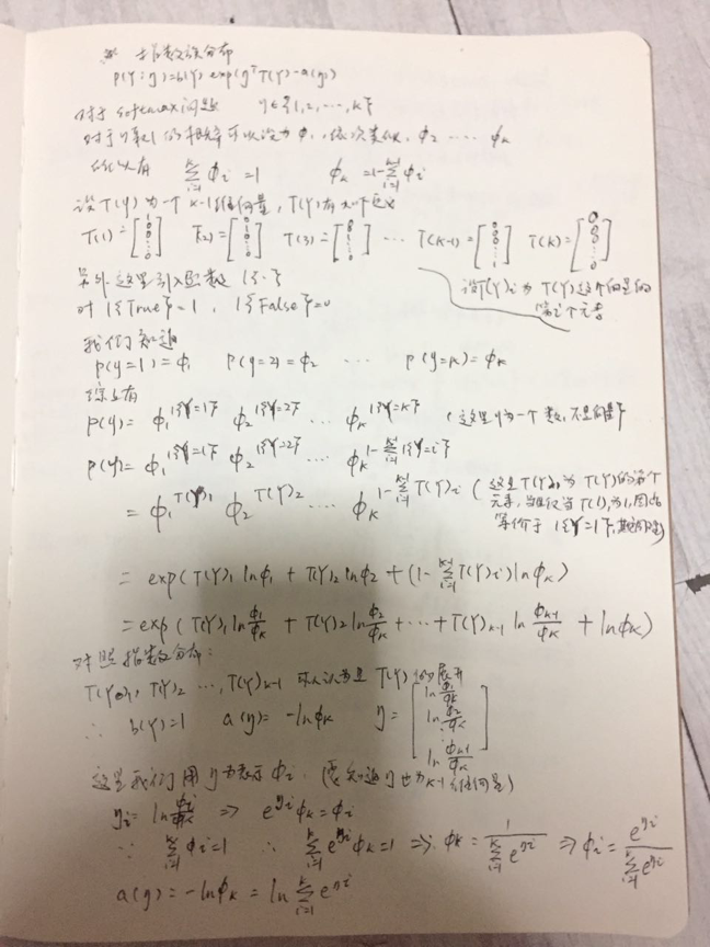
在进行下一步推导前,我们先定义部分辅助函数。我们这里事先定义一个k-1维向量\(T(y)\),这里具体对应于指数族分布的\(T(y)\),具体定义如下:

$$T(1) = \left[ \begin{gathered} 1 \hfill \\\ 0 \hfill \\\ 0 \hfill \\\ ... \hfill \\\ 0 \hfill \\ \end{gathered} \right],T(2) = \left[ \begin{gathered} 0 \hfill \\\ 1 \hfill \\\ 0 \hfill \\\ ... \hfill \\\ 0 \hfill \\ \end{gathered} \right],T(3) = \left[ \begin{gathered} 0 \hfill \\\ 0 \hfill \\\ 1 \hfill \\\ ... \hfill \\\ 0 \hfill \\\ \end{gathered} \right],...,T(k - 1) = \left[ \begin{gathered} 0 \hfill \\\ 0 \hfill \\\ 0 \hfill \\\ ... \hfill \\\ 1 \hfill \\ \end{gathered} \right],T(k) = \left[ \begin{gathered} 0 \hfill \\\ 0 \hfill \\\ 0 \hfill \\\ ... \hfill \\\ 0 \hfill \\ \end{gathered} \right]$$

我们定义\(T(y) _1\)表示的\(T(y)\)第一个元素,其他依次类推。

然后再引入一个函数,具体定义如下:

$$1\{ true\} = 1$$ $$1\{ false\} = 0$$

可以通过带入值的方式验证上式。

2 模型推导

在softmax中,我们知道\(y \in \{ 1,2,…,k\}\)。我们设置\(y=1\)的概率为\(\phi _1\),
类似的有\(y=k\)的概率为\(\phi _k\),并且我们轻易得到如下公式:

$$\sum\limits _{i = 1}^k {\phi _i} = 1$$ $${\phi _k} = \sum\limits _{i = 1}^{k - 1}{\phi _i}$$

由于我们已经知道\(p(y = i) = {\phi _i}\),综上可以得到:

$$p(y) = \phi _1^{1\{ y = 1\} }\phi _2^{1\{ y = 2\} }...\phi _k^{1\{ y = k\} } = \phi _1^{1\{ y = 1\} }\phi _2^{1\{ y = 2\} }...\phi _k^{1 - \sum\limits _{i = 1}^{k - 1} {1\{ y = i\} } } = \phi _1^{T{(y)} _1}\phi _2^{T{{(y)} _2}}...\phi _k^{1 - \sum\limits _{i = 1}^{k - 1} {T{(y)} _i} }$$ $$p(y) = \exp (T{(y) _1}\ln {\phi _1} + T{(y) _2}\ln {\phi _2} + ... + (1 - \sum\limits _{i = 1}^{k - 1} {T{{(y)} _i}} )\ln {\phi _k})$$ $$p(y) = \exp (T{(y) _1}\ln \frac{\phi _1}{\phi _k} + T{(y) _2}\ln \frac{\phi _2}{\phi _k} + ... + T{(y) _{k - 1}}\ln \frac{\phi _{k - 1}}{\phi _k} + \ln {\phi _k})$$

我们对照指数族分布,其中\(T(y)\)我们已经定义,可以得到其他参数如下:

$$b(y) = 1$$ $$a(\eta ) = - \ln {\phi _k}$$ $$\eta = \left[ \begin{gathered} \ln \frac{\phi _1}{\phi _k} \hfill \\\ \ln \frac{\phi _2}{\phi _k} \hfill \\\ ... \hfill \\\ \ln \frac{\phi _{k - 1}}{\phi _k} \hfill \\\ \end{gathered} \right]$$

我们用\(\eta\)来表示\(\phi\),目标是将我们的问题归整为一个变量的问题,从而更容易计算。对上面向量拆开计算得到:

$${\eta _i} = \ln \frac{\phi _i}{\phi _k}$$

继而可以转化为:

$${\eta _i} = \ln \frac{\phi _i}{\phi _k}$$

又由于我们已知\(\sum\limits _{j = 1}^k {\phi _j} = 1\),所以有:

$$\sum\limits _{i = 1}^k {e^{\eta _i}{\phi _k}} = 1$$

继而有:

$${\phi _k} = \frac{1}{\sum\limits _{j = 1}^k {e^{\eta _j}}}$$

最后我们可以得到:

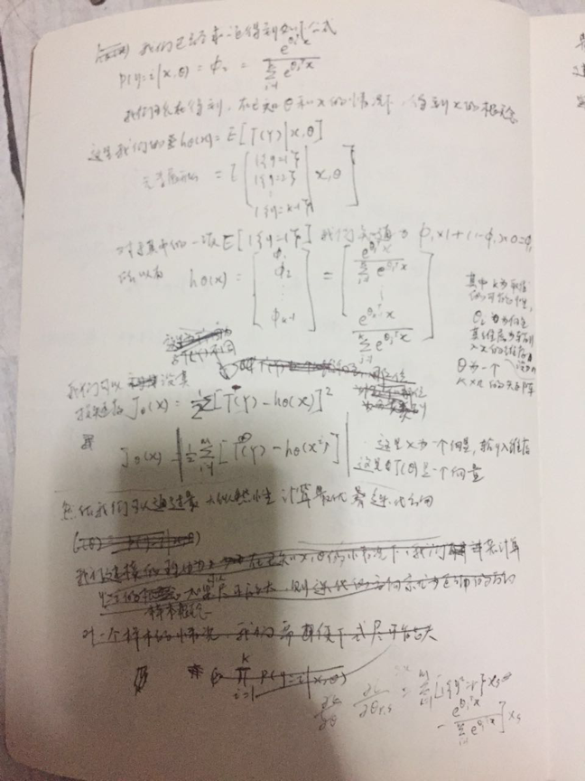
$${\phi _i} = \frac{e^{\eta _i}}{\sum\limits _{j = 1}^k {e^{\eta _j}}}$$

由于指数组分布假设是关于输入的线性函数,所以得到在已知\(x\)和\(\theta\)的情况下\(y=i\)的概率的公式,如下:

$$p(y = i|x,\theta ) = {\phi _i} = \frac{e^{\eta _i}}{\sum\limits _{j = 1}^k {e^{\eta _j}}} = \frac{e^{\theta _i^Tx}}{\sum\limits _{j = 1}^k {e^{\theta _j^Tx}}}$$

这里我们可以得到\({h_\theta }(x)\),如下:

$${h_\theta }(x) = E[T(y)|x,\theta ] = E[\left( \begin{gathered} 1\{ y = 1\} \hfill \\\ 1\{ y = 2\} \hfill \\\ ... \hfill \\\ 1\{ y = k - 1\} \hfill \\\ \end{gathered} \right)|x,\theta ]$$ $${h_ \theta }(x) = E[\left( \begin{gathered} {\phi _1} \hfill \\\ {\phi _2} \hfill \\\ ... \hfill \\\ {\phi _{k - 1}} \hfill \\\ \end{gathered} \right)|x,\theta ] = \left( \begin{gathered} \frac{e^{\theta _1^Tx}}{\sum\limits _{j = 1}^k {e^{\theta _j^Tx}}} \hfill \\\ \frac{e^{\theta _2^Tx}}{\sum\limits _{j = 1}^k {e^{\theta _j^Tx}}} \hfill \\\ ... \hfill \\\ \frac{e^{\theta _{k - 1}^Tx}}{\sum\limits _{j = 1}^k {e^{\theta _j^Tx}}} \hfill \\\ \end{gathered} \right)$$

其中,\(k\)为取值的可能集合的大小,\(\theta\)为一个\(k*n\)的矩阵。

到这里我们可以定义我们的损失函数了,如下:

$$J(x) = \frac{1}{2}\sum\limits _{i = 1}^m {{(T(y) - {h _\theta }(x))}^2}$$

上式是一个向量,我们可以对这个向量继续求平方和,来衡量准确度,如下:

$$J(x) = \frac{1}{2}\sum\limits _{i = 1}^m {|{{(T(y) - {h _\theta }(x))}^2}|}$$

损失函数已经定义完成,我们就有了算法的截止条件了。接下来就是找到算法的最优迭代方向,也就是计算其偏导数了。

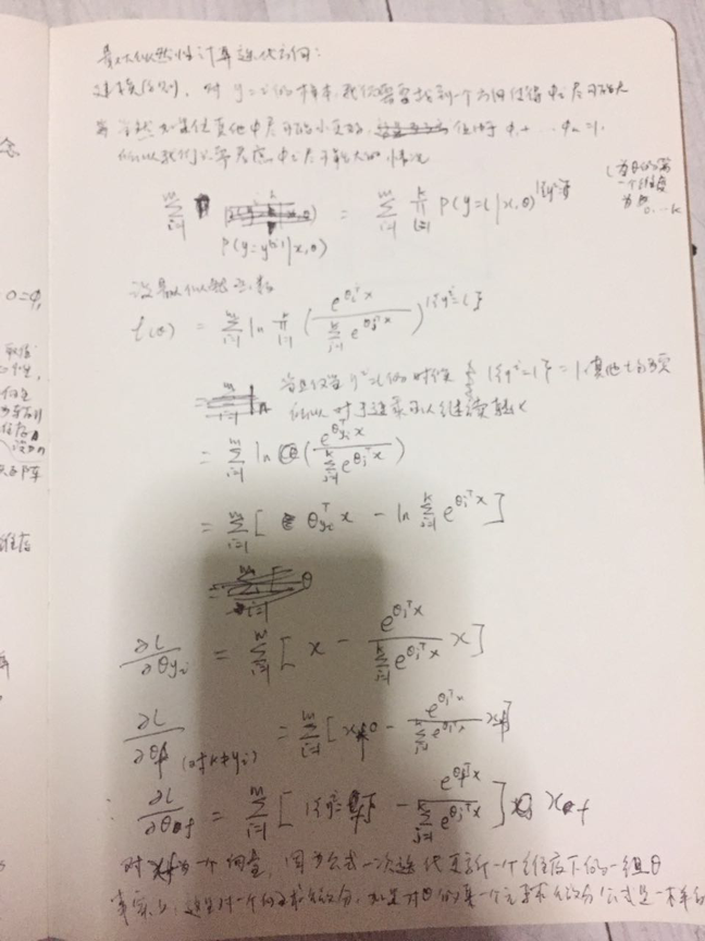
我们使用最大释然性来计算迭代方向。建模的原则是:对于一个已知\(y=i\)的样本\((x,y)\),我们需要找到一个方向去迭代\(\theta\),使得\(\phi _i\)尽可能大,使得其他\(\phi\)尽可能小。当然由于所有\(\phi\)之和为1,所以我们只需要保证\(\phi _i\)尽可能大即可。因此,在已经的\(m\)个样本的情况下,我们只需要保证下面的式子最大:

$$\sum\limits _{i = 1}^m {p(y = {y^i}|x,\theta )} = \sum\limits _{i = 1}^m {\prod\limits _{l = 1}^k {p{(y = l|x,\theta )}^{1\{ {y^i} = l\}}} }$$

取自然对数后,我们定义最大似然函数:

$$l(\theta ) = \sum\limits _{i = 1}^m {\ln \prod\limits _{l = 1}^k {(\frac{e^{\theta _l^Tx}}{\sum\limits _{j = 1}^k {e^{\theta _j^Tx}}})^{1\{{y^i} = l\}}}}$$

当且仅当\({y^i} = l\)的时候, \({1{yi=l\} = 1})。其他值为0,我们可以将连乘转化,如下:

$$l(\theta ) = \sum\limits _{i = 1}^m {\ln (\frac{e^{\theta _{y^i}^Tx}}{\sum\limits _{j = 1}^k {e^{\theta _j^Tx}}})} = \sum\limits _{i = 1}^m {\ln [\theta _{y^i}^Tx - \ln \sum\limits _{j = 1}^k {e^{\theta _j^Tx}}]} $$

然后对其求偏导数,对\(y _i=f\)的时候后有:

$$\frac{\partial l(\theta )}{\partial {\theta _f}} = \sum\limits _{i = 1}^m {\ln [{x _f} - \frac{e^{\theta _f^Tx}{x _f}}{\sum\limits _{j = 1}^k {e^{\theta _j^Tx}}}]}$$

对\({y_i} \ne f\)的时候,有:

$$\frac{\partial l(\theta )}{\partial {\theta _f}} = \sum\limits _{i = 1}^m {\ln [0 - \frac{e^{\theta _f^Tx}{x _f}}{\sum\limits _{j = 1}^k {e^{\theta _j^Tx}}}]}$$

综上,可以得到:

$$\frac{\partial l(\theta )}{\partial {\theta _f}} = \sum\limits _{i = 1}^m {\ln [1\{ {y^i} = f\} - \frac{e^{\theta _f^Tx}}{\sum\limits _{j = 1}^k {e^{\theta _j^Tx}}}]{x _f}} = \sum\limits _{i = 1}^m {\ln [1\{{y^i} = f\} - {\phi _f}]{x _f}}$$

\(x _f\)是一个向量,因为公式一次迭代更新一个维度下的一组\(\theta\)。事实上,这里是一个向量求微分。如果我们对的某个元素\(\theta\)进行微分,我们依然能够得到这个公式。

3 实际问题的解决

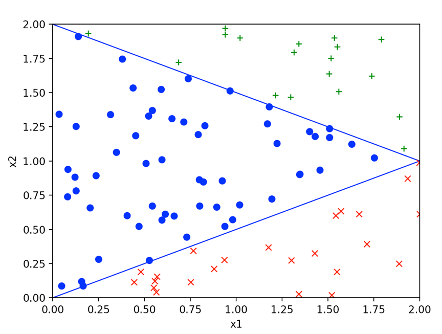
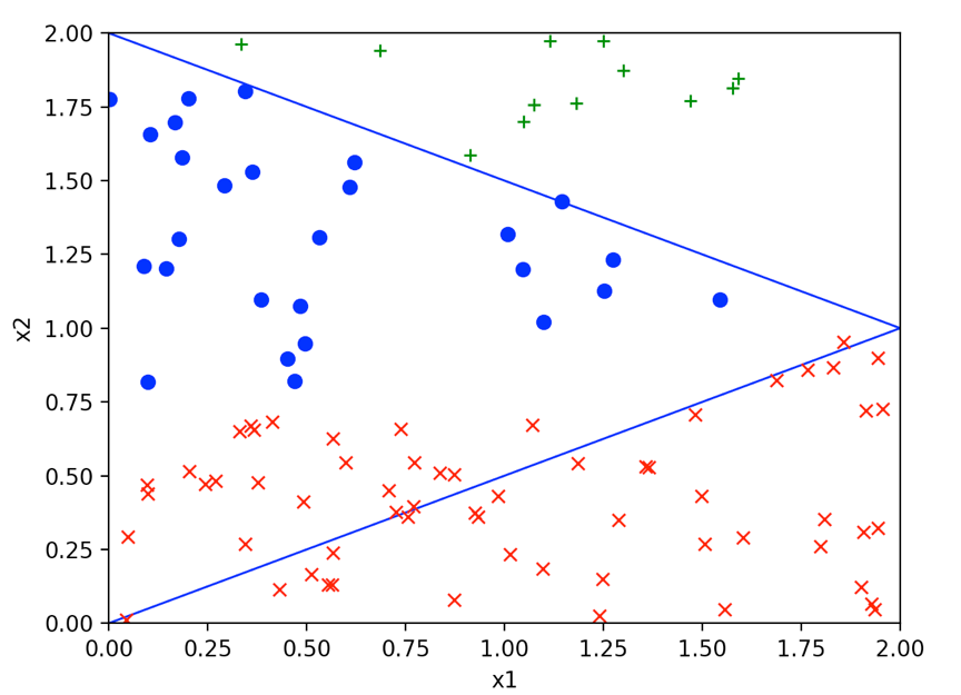
我们随机制造一组数据,在\(2*2\)的空间内使用直线\({x _2} = 0.5*{x _1}\)和直线\({x _2} = -0.5*{x _1}+2\)具体的分类如下:

根据之前的推导,编写如下代码:

1
2
3
4
5
6
7
8
9
10
11
12
13
14
15
16
17
18
19
20
21
22
23
24
25
26
27
28
29
30
31
32
33
34
35
36
37
38
39
40
41
42
43
44
45
46
47
48
49
50
51
52
53
54
55
56
57
58
59
60
61
62
63
64
65
66
67
68
69
70
71
72
73
74
75
76
77
78
79
80
81
82
83
84
85
86
87
88
89
90
91
92
93
94
95
96
97
98
99
100
101
102
103
104
105
106
107
108
109
110
111
112
113
114
115
116
117
118
119
120
121
122
123
124
125
126
127
128
129
130
131
132
133
134
135
import random
import math
import numpy as np
from matplotlib import pyplot as plt
from matplotlib.lines import Line2D

g_x_arr=[[1, 0.035, 1.344], [1, 0.662, 0.598], [1, 1.791, 1.889], [1, 0.158, 0.12], [1, 1.55, 1.835], [1, 2.0, 0.613], [1, 1.176, 0.368], [1, 0.564, 0.043], [1, 1.559, 1.507], [1, 1.998, 0.988], [1, 0.082, 0.941], [1, 0.542, 1.371], [1, 0.542, 0.671], [1, 1.34, 1.856], [1, 0.049, 0.089], [1, 1.933, 0.871], [1, 1.753, 1.024], [1, 0.315, 1.341], [1, 0.829, 1.26], [1, 0.686, 1.721], [1, 1.222, 1.129], [1, 0.55, 0.075], [1, 0.767, 0.346], [1, 1.516, 1.752], [1, 1.347, 0.905], [1, 0.127, 0.782], [1, 1.169, 1.272], [1, 1.301, 0.273], [1, 0.081, 0.739], [1, 0.203, 0.658], [1, 0.347, 1.064], [1, 0.793, 1.193], [1, 1.428, 0.326], [1, 0.509, 0.983], [1, 0.12, 0.884], [1, 0.251, 0.282], [1, 0.73, 0.445], [1, 1.889, 1.323], [1, 1.314, 1.795], [1, 1.297, 1.467], [1, 1.669, 0.613], [1, 0.753, 0.114], [1, 0.94, 1.972], [1, 0.738, 1.603], [1, 1.508, 1.237], [1, 0.979, 0.572], [1, 0.128, 1.254], [1, 0.569, 0.155], [1, 0.88, 0.211], [1, 0.405, 0.603], [1, 1.02, 1.9], [1, 0.438, 1.535], [1, 1.506, 1.638], [1, 1.712, 0.394], [1, 0.556, 0.124], [1, 0.444, 0.115], [1, 0.595, 1.009], [1, 0.165, 0.089], [1, 1.57, 0.634], [1, 1.429, 1.181], [1, 0.8, 0.671], [1, 1.914, 1.091], [1, 0.594, 0.569], [1, 0.935, 0.277], [1, 0.47, 0.522], [1, 0.94, 1.924], [1, 0.194, 1.933], [1, 0.612, 0.613], [1, 0.236, 0.894], [1, 1.888, 0.251], [1, 1.548, 0.191], [1, 1.543, 0.603], [1, 1.521, 0.02], [1, 0.923, 0.856], [1, 0.649, 1.31], [1, 0.379, 1.746], [1, 1.345, 0.902], [1, 0.937, 0.524], [1, 1.018, 0.68], [1, 1.738, 1.623], [1, 1.534, 1.9], [1, 0.139, 1.911], [1, 1.508, 1.173], [1, 0.798, 0.865], [1, 0.451, 1.186], [1, 1.63, 1.123], [1, 0.82, 0.848], [1, 1.213, 1.48], [1, 0.894, 0.664], [1, 1.456, 0.934], [1, 0.59, 1.525], [1, 0.522, 1.329], [1, 1.179, 1.396], [1, 0.527, 0.273], [1, 1.399, 1.215], [1, 0.966, 1.514], [1, 1.341, 0.028], [1, 0.479, 0.191], [1, 1.193, 0.724], [1, 0.714, 1.285]]
g_Ty_arr=[[0, 0], [0, 0], [0, 1], [0, 0], [0, 1], [1, 0], [1, 0], [1, 0], [0, 1], [1, 0], [0, 0], [0, 0], [0, 0], [0, 1], [0, 0], [1, 0], [0, 0], [0, 0], [0, 0], [0, 1], [0, 0], [1, 0], [1, 0], [0, 1], [0, 0], [0, 0], [0, 0], [1, 0], [0, 0], [0, 0], [0, 0], [0, 0], [1, 0], [0, 0], [0, 0], [0, 0], [0, 0], [0, 1], [0, 1], [0, 1], [1, 0], [1, 0], [0, 1], [0, 0], [0, 0], [0, 0], [0, 0], [1, 0], [1, 0], [0, 0], [0, 1], [0, 0], [0, 1], [1, 0], [1, 0], [1, 0], [0, 0], [0, 0], [1, 0], [0, 0], [0, 0], [0, 1], [0, 0], [1, 0], [0, 0], [0, 1], [0, 1], [0, 0], [0, 0], [1, 0], [1, 0], [1, 0], [1, 0], [0, 0], [0, 0], [0, 0], [0, 0], [0, 0], [0, 0], [0, 1], [0, 1], [0, 0], [0, 0], [0, 0], [0, 0], [0, 0], [0, 0], [0, 1], [0, 0], [0, 0], [0, 0], [0, 0], [0, 0], [0, 0], [0, 0], [0, 0], [1, 0], [1, 0], [0, 0], [0, 0]]
g_y_arr=[2, 2, 1, 2, 1, 0, 0, 0, 1, 0, 2, 2, 2, 1, 2, 0, 2, 2, 2, 1, 2, 0, 0, 1, 2, 2, 2, 0, 2, 2, 2, 2, 0, 2, 2, 2, 2, 1, 1, 1, 0, 0, 1, 2, 2, 2, 2, 0, 0, 2, 1, 2, 1, 0, 0, 0, 2, 2, 0, 2, 2, 1, 2, 0, 2, 1, 1, 2, 2, 0, 0, 0, 0, 2, 2, 2, 2, 2, 2, 1, 1, 2, 2, 2, 2, 2, 2, 1, 2, 2, 2, 2, 2, 2, 2, 2, 0, 0, 2, 2]

def phi(i,theta,x):
theta_n = len(theta)
numerator = math.exp(np.dot(theta[i], x))
denominator = 0;
for j in range(theta_n): # maybe need to optimize
denominator = denominator + math.exp(np.dot(theta[j],x))
return numerator/denominator

def h_theta(theta,x):
theta_n = len(theta)
ret = []
for i in range(theta_n):
ret.append(phi(i,theta,x))
return ret

def one(y,i):
if y == i:
return 1
else:
return 0

def derl(f,x_arr,y_arr,theta):
# 0.
# f is the dimension to calc the partial derivative
# 1. calc the size
# theta_n is the size of theta, equals to the length of Ty' result set -1 .Here, equals lenght of {0,1,2} = 3-1 =2
# m is the sum of samples
# x_n is the dimension of the input variable 'x' + 1 (for x_0 =1). Here is 2 + 1 = 3
theta_n = len(theta)
m = len(x_arr)
x_n = len(x_arr[0])
# initial the output variable sum.Here is a vector, and the length of this vector is x_n
sum = []
for x_dim_index in range(x_n):
sum.append(0)
# 2. calc the partial derivative
for i in range(x_n):
sum[i] = 0
for j in range(m):
sum[i]=sum[i]+(one(y_arr[j],f)-phi(f,theta,x_arr[j]))*x_arr[j][i]
sum[i]=sum[i]/m
#sum=plus_vector(sum,theta[f],0.1)
return sum

def plus_vector(arr1,arr2,a):
return [x + a * y for x, y in zip(arr1, arr2)]

def update(theta,a,x_arr,y_arr):
theta_n = len(theta)
for i in range(theta_n):
theta[i]=plus_vector(theta[i],derl(i, x_arr,y_arr,theta),a)
return theta

def judge1(theta,x_arr,y_arr_vector,limit,debug):
j_theta = J(theta,x_arr,y_arr_vector)
if j_theta < limit:
return True
if debug:
print("|J_theta(x)| = ", j_theta,"\n")
return False

def J(theta,x_arr,y_arr_vector):
sum=0
m = len(x_arr)
y_len = len(y_arr_vector[0])
for i in range(m):
for j in range(y_len):
sum = sum + (phi(j,theta,x_arr[i]) - y_arr_vector[i][j])**2
return sum

def calTheVaule():
#theta=[[theta_1_1,theta_1_2],[theta_2_1,theta_2_2],[theta_3_1,theta_3_2]]
theta = [[1,1,1],[1,1,1],[1,1,1]]
a = 1
count = 0
while 1:
if judge1(theta,g_x_arr,g_Ty_arr,1,True):
break
theta=update(theta,a,g_x_arr,g_y_arr)
count = count + 1
print("count=",count,"theta=",theta)

def calcIndex(theta,x):
phi0 = phi(0,theta,x)
phi1 = phi(1,theta,x)
phi2 = phi(2,theta,x)
if phi0 >= phi1 and phi0 >=phi1:
return 0
elif phi1>= phi0 and phi1 >= phi2:
return 1
else:
return 2

def testValue():
# limit =1, count = 33844
theta = [[17.418683742474045, 13.989348587756815, -37.731307869980014],[-33.56035031194091, 1.3797244978249763, 34.095843086377855],[19.97548491920147, -11.65484983882828, 7.628008093823735]]
samples = 100
figure, ax = plt.subplots()
# 设置x,y值域
ax.set_xlim(left=0, right=2)
ax.set_ylim(bottom=0, top=2)
# 两条line的数据
(line1_xs, line1_ys) = [(0, 2), (0, 1)]
(line2_xs, line2_ys) = [(0, 2), (2, 1)]
# 创建两条线,并添加
ax.add_line(Line2D(line1_xs, line1_ys, linewidth=1, color='blue'))
ax.add_line(Line2D(line2_xs, line2_ys, linewidth=1, color='blue'))
for i in range(samples):
x_0 = random.randint(0,2000)/1000
x_1 = random.randint(0,2000)/1000
index = calcIndex(theta,[1,x_0,x_1])
if index == 0:
plt.plot(x_0, x_1, 'b--', marker='x', color='r')
elif index == 1:
plt.plot(x_0, x_1, 'b--', marker='+', color='g')
else:
plt.plot(x_0, x_1, 'b--', marker='o', color='b')
plt.xlabel("x1")
plt.ylabel("x2")
plt.plot()
plt.show()

if __name__== "__main__":
#calTheVaule()
testValue()

经过33844次迭代之后,我们得到\(\theta\) = [[17.418683742474045, 13.989348587756815, -37.731307869980014],[-33.56035031194091, 1.3797244978249763, 34.095843086377855],[19.97548491920147, -11.65484983882828, 7.628008093823735]]

迭代的次数越多数据会越准确,这里迭代了上三万次,实际上可以通过牛顿法来减少迭代的次数,这里就不再重新代码了,牛顿法可以参见前面的文章。

然后,我们随机制造一组值,看看分类效果,具体如下:

附录 公式推导手写版